Graph of the Relations between Objects in the diffgeom Module

This graph, besides showing naively in a rather simplistic way the structure of the theory of differential geometry (and most of what I have implemented in the diffgeom module), brings attention to the one non-trivial part of the module on which I have spent most of my time lately. Namely, implementing covariant derivatives.

All directional derivatives are defined as a limiting procedure on a transport operator. Besides the Lie derivatives which use a certain transport operator that is easy to express in a coordinate free way, all other derivatives, called covariant derivatives have to be expressed using something called Christoffel symbols. And these are the ugly coordinate-dependent sources of pain, as the module structure becomes very cumbersome when such dependence must be accounted for. Thankfully, I think I have found a nice way to implement them in a new CovariantDerivativeOperator class on its own, that will contain all the logic in the same way in which the Base*Field classes do it. This will also require rewrite of the LieDerivative into a LieDerivativeOperator class.

The diffgeom Module – Status Report

I have written already a few posts about the theory behind the module, the structure of the module, etc. However, besides some rare examples, I have not described in much details how the work progresses. So here is a short summary (check the git log for more details):

  • The basics about coordinate systems and fields are already in. There are numerous issues with all the simplify-like algorithms inside SymPy, however they are slowly ironed out.
  • Some simplistic methods for work with integral curves are implemented.
  • The basics of tensor/wedge products are in. Many simplification routines can be added. Contraction between tensor products and vectors is possible (special case of “lowering of an index”).
  • Over-a-map, pushforwards and pullbacks are not implemented yet.
  • Instead of them I have focused my work on derivatives and curvature tensors. For the moment work on these can be done in a limited coordinate-dependent way. A longer post explaining the theory is coming and with it an implementation slightly less dependent on coordinates (working with Christoffel symbols is a pain).
  • Hodge star operator – still not implemented.

An example that I want to implement is a theorem that in irrotational cosmology isotropy implies homogeneity. Doing this will be the first non-trivial example in this module.

A serendipitous detour from the project was my work on the differential equations solver. Aaron had implemented a very thorough solver for single equations. I had tried to extend it in a few simple ways in order to work with systems of ODEs and initial conditions. However this led me to Jordan forms of matrices, generalized eigenvectors and a bunch of interesting details on which I work in my free time (especially this week).

Form Fields and Vector Fields do not form a Vector Space

Form fields or vector fields over a manifold (as opposed to forms and vectors) do not form a vector space. They form a module.

The difference is that the scalars of a vector space form an algebraic field while the scalars of a module form a ring. For us humans (as opposed to “those higher beings that I do not understand (a.k.a. mathematicians)”) this means that the scalars in the vector field can divide each other while the scalars in the spaces spanned by fields (i.e. a module) can not.

And just so we all can become even more confused: This has nothing to do with the fact that the “components” of each form field or vector field in certain basis are functions, i.e. themselves elements of a vector space with infinite number of dimensions.

The first way to see this module-not-a-vector-space characteristic is by showing directly that the scalars that form the “coordinate components” of a vector field can not always be divided, even if they are not identically zero. Take, for instance the, manifold \mathbb{R}^2 with the polar coordinate system and look at the vector \begin{bmatrix} r \\ r\cos(\theta) \end{bmatrix}. The “scalars” are r and r\cos(\theta). Obviously we can not divide the former by the latter because it will be undefined at \theta=\frac{\pi}{2}+n\pi.

Another, more amusing way to show that the space spanned by these fields is not a vector space is to explicitly show that a property expected from vector spaces is not fulfilled. Namely, that in n dimensions an n-uple of linearly independent elements forms a basis. However, in the case of fields over a manifold we can easily have a number of fields that are linearly independent over the manifold as a whole, and are at the same time linearly dependent (or simply equal to zero) on a subdomain. Hence, we have an n-uple of linearly independent fields that can not be linearly combined to represent another arbitrary field.

Objects Implemented in the diffgeom Module

This post provides a summary of all mathematical types of expression implemented in the diffgeom module. I have chosen not to mention any python classes or other implementation details at all. This table shows how an object expected by the user to be of certain mathematical type operates on another object. If the expectations of a user familiar with differential geometry do not meet the actual implementation, this is a bug in the implementation.

The Argument
point scalar field vector field 1-form field higher form field
The Operator scalar field scalar NA NA NA NA
vector field NA scalar field NA NA NA
1-form field (linear combination of differentials of scalar fields) NA NA scalar field NA NA
higher form field (linear combination of tensor products of lower form fields) NA NA it takes a tuple of vector fields and returns a scalar field NA NA
commutator of vector fields Behaves as a regular vector field.
Lie derivative (the argument is “called” on construction time) NA You specify the object to be derived on creation. The Lie derivative of any object is an object of the same type.

The Schwarzschild Solution

An “easy” solution to the Einstein equation (in free space) is the spherically symmetric Schwarzschild solution. The pdf bellow shows how one can use the diffgeom module in order to get the equations describing this solution.

One starts with the most general spherically symmetrical metric and by using Einstein equation R_{\mu \nu}=0 deduces the equations that must be fulfilled by the components of the metric (in the chosen basis).

schwarzschild.pdf

Tensor vs Tensor Field, Basis vs Coordinate System

In most of my posts that discuss the SymPy diffgeom module I do not try to make a distinction between a tensor and a tensor field, as it is usually obvious from the context. However, it would be nice to spell it out at least once.

I have two favorite ways to define a tensor/tensor field: either as an object with a representation (in the form of a multidimensional array) that transforms in a precise way when one switches from one basis to another, or instead as (sum of) tensor products of some vectors and 1-forms (i.e. an element of some tensor product of the vector space and its dual).

In Terms of Transformation Rules

With regard to the first definition, Wikipedia has this to say:

A tensor of type (n, m−n) is an assignment of a multidimensional array T^{i_1\dots i_n}_{i_{n+1}\dots i_m}[\mathbf{f}] to each basis f = (e_1,...,e_N) such that, if we apply the change of basis \mathbf{f}\mapsto \mathbf{f}\cdot R = \left( R_1^i \mathbf{e}_i, \dots, R_N^i\mathbf{e}_i\right) then the multidimensional array obeys the transformation law T^{i_1\dots i_n}_{i_{n+1}\dots i_m}[\mathbf{f}\cdot R] = (R^{-1})^{i_1}_{j_1}\cdots(R^{-1})^{i_n}_{j_n} R^{j_{n+1}}_{i_{n+1}}\cdots R^{j_{m}}_{i_{m}}T^{j_1,\ldots,j_n}_{j_{n+1},\ldots,j_m}[\mathbf{f}] .

A tensor field then is a way to map a tensor to each point of a manifold (the tensor is wrt the tangent space at that point).

When we switch from tensors to tensor fields a new object becomes important: the coordinate system. Before proceeding, one must know what a manifold and a tangent space mean. Then we can illuminate the relation between what one calls a “basis” when speaking about tensors and the “coordinate system” in the context of tensor fields. Firstly, a coordinate system gives a way to continuously map a tuple of numbers to a point on the manifold. This continuous map is what physicist love to work with (Cartesian or polar coordinates for instance). The nice thing is that each coordinate system brings with itself a canonical basis for each point of the manifold.

What can be confusing, is that the basis can change from point to point. For example, one can take the R^2 manifold that has R^2 as its tangent space. Take for instance two points (x=1, y=0) and (x=0, y=1). The basis vectors in the Cartesian coordinate system are the same for both points: (e_x, e_y). However in the polar coordinate system the basis vectors for the first point are (e_x, e_y) and (e_y, -e_x) for the second point.

Anyway, the only thing that changes in the definition, is that the change-of-basis matrix mentioned above now depends on the coordinate systems.

\hat{T}^{i_1\dots i_n}_{i_{n+1}\dots i_m}(\bar{x}_1,\ldots,\bar{x}_k) =  \frac{\partial \bar{x}^{i_1}}{\partial x^{j_1}}  \cdots  \frac{\partial \bar{x}^{i_n}}{\partial x^{j_n}}  \frac{\partial x^{j_{n+1}}}{\partial \bar{x}^{i_{n+1}}}  \cdots  \frac{\partial x^{j_m}}{\partial \bar{x}^{i_m}}  T^{j_1\dots j_n}_{j_{n+1}\dots j_m}(x_1,\ldots,x_k)

In Terms of Tensor Products

I prefer this definition, as it relies on the geometrical meaning of vectors and forms. According to Wikipedia, one can express it as:

A type (n, m) tensor T is defined as a map T: \underbrace{ V^* \times\dots\times V^*}_{n \text{ copies}} \times \underbrace{ V \times\dots\times V}_{m \text{ copies}} \rightarrow \mathbf{R} 
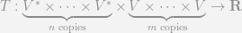
, where V is a vector space and V* is the corresponding dual space of covectors, which is linear in each of its arguments.

One can again try to translate this to the case of tensor fields. The straightforward way is just to say that this map is parametrized, thus it depends on which point on the manifold it is evaluated.

However, a more “geometrical” approach would be to keep the part about “a tensor field is the sum of tensor products of vector fields and 1-form fields” but define vector fields and 1-form fields “geometrically”. Vector fields become differential operators over the manifold instead of maps to elements of the tangent space and 1-forms are defined in terms of differentials instead of duals of vectors.

The Magic

The magic is that this parametrization in terms of tuples of real numbers (a coordinate system) brings automatically a canonical basis and and the transformation matrix for change of basis. Hence defining a coordinate system provides a basis for free. Otherwise the generalization of the first definition would have been clumsier.

Part 1: What is a Tensor and How is it Implemented in the diffgeom SymPy module?

The Math

The notion of “a tensor” is commonly defined in two different ways. The first definition goes roughly like this (“roughly” means “do not tell this to your math teacher”):

A tensor is a geometrical object that can be represented in some coordinate system as an n-dimensional array (it is not the array itself). The quantities in that array depend on the coordinate system in which the representation is done, however there is a precise rule on how these quantities change if we switch to another coordinate system. It is this rule that defines what a tensor (and in particular a vector or a 1-form) is.

The other definition, less used by physicists and more used by mathematicians is (again roughly) the following:

A tensor is the sum of tensor products of forms and vectors. Forms and vectors are themselves given nice geometrical definitions.

It is this second definition that is used in the diffgeom SymPy module. Naturally, we need to define “tensor product”, “vector” and “form” in order to use this definition. Indeed, the structure of the module follows closely these mathematical definitions.

Disclaimer: I have used and will use the words tensor and tensor field interchangeably. In order for this post to make any sense to you, ensure that you understand the difference and are able to find out the exact meaning from the context. The same goes also for vector / vector field and form / form field.

The Implementation

To create the mathematical structure of differential geometry or its implementation in a CAS like SymPy we need to build up the ladder of object definitions. Each new and more interesting notion will depend on the definition of the previous. Hence we start with the boilerplate object “Manifold” and on it we define a “Patch” (the diffgeom module implements all this boilerplate for commonly used manifold, however in order to explain how it works, we will redo everything from scratch):

m = Manifold('my_manifold', 2) # A 2D manifold called 'my_manifold'
p = Patch('my_patch', m) # A patch called 'my_patch'
 

The first object that does something marginally interesting is the “Coordinate System”. Its role is to permit the parametrization of points on the patch by a tuple of numbers:

cs_r = CoordSystem('R', p) # A coordinate system called 'R' (for rectangular)
point = cs_r.point([1,1]) # A point with coordinates (1, 1)

If you have two or more coordinate systems you can tell the computer how to transform a tuple of numbers from one system to another:

cs_p = CoordSystem('P', p)
cs_r.connect_to(cs_p, [x, y], [sqrt(x**2+y**2), atan2(y,x)])
cs_p.connect_to(cs_r, [r, t], [r*cos(t), r*sin(t)], inverse=False)
# Now the point instances know how to transform their coordinate tuples:
point.coords(cs_p)
# output:
#⎡  ___⎤
#⎢╲╱ 2 ⎥
#⎢     ⎥
#⎢  π  ⎥
#⎢  ─  ⎥
#⎣  4  ⎦

However, differential geometry is not about calculating coordinates of points in different systems. It is about working with fields. Thus, we will focus on a single coordinate system from now on, and to be explicit about its complete independence of whether we want rectangular or other coordinates, we will just call it ‘c’ and leave it unconnected to other coordinate systems.

c = CoordSystem('c', p)

Scalar Field

We continue to build up our ladder of definitions in order to obtain a more interesting and useful theory/implementation. The next step is the “scalar field”. A scalar field is a mapping from the manifold (the set of points) to the real numbers (yes, just reals (maybe complex), the rest brings unnecessary complexity). Each coordinate system brings with itself the basic scalar fields (i.e. coordinate functions), that correspond to the mappings from a point to an element of its coordinate tuple. These basic scalar fields are implemented internally as BaseScalarField instances (this is however invisible to the user).

 c.coord_functions()
# output: [c₀, c₁]
point = c.point([a, b])
c.coord_function(0)(point)
# output: a

You can build more complicated fields by using the base scalar fields. This does not produce an instance of some new ScalarField class. The BaseScalarField instances just become a part of the expression tree of an ordinary Expr instance (the base for building expressions in SymPy).

c0, c1 = c.coord_functions()
field = f(c0, 3*c1)/sin(c0)*c1**2
f
# output:
#               -1       2
#f(c₀, 3⋅c₁)⋅sin  (c₀)⋅c₁
field(point)
# output:
# 2
#b ⋅f(a, 3⋅b)
#────────────
#   sin(a)

Vector Field

Then comes the vector field which is defined as an element of the set of differential operators over the scalar fields. All elements of this set can be build up as linear combinations of base vector fields. The base vector fields correspond to the partial derivatives with respect to the base scalar fields. They are implemented in the BaseVectorField class, which also is invisible to the user.

c.base_vectors()
# output: [∂_c_0, ∂_c_1]
e_c0, e_c1 = c.base_vectors()
e_c0(c0)
# output: 1
e_c0(c1)
# output: 0

One can also use more complicated fields (again, no need for new VectorField class, just being part of the expression tree of Expr):

v_field = c1*e_c0 + f(c0)*e_c1
v_field
# output: f(c₀)⋅∂_c_1 + c₁⋅∂_c_0
s_field = g(c0, c1)
v_field(s_field)
# output:
#      ⎛ d            ⎞│           ⎛ d            ⎞│
#f(c₀)⋅⎜───(g(c₀, ξ₂))⎟│      + c₁⋅⎜───(g(ξ₁, c₁))⎟│
#      ⎝dξ₂           ⎠│ξ₂=c₁      ⎝dξ₁           ⎠│ξ₁=c₀
v_field(s_field)(point)
# output:
#  ⎛ d           ⎞│            ⎛ d           ⎞│
#b⋅⎜───(g(ξ₁, b))⎟│     + f(a)⋅⎜───(g(a, ξ₂))⎟│
#  ⎝dξ₁          ⎠│ξ₁=a        ⎝dξ₂          ⎠│ξ₂=b

1-Form Field and Differential

The final ingredient needed for the basis of differential geometry is the 1-form field. A 1-form field is a linear mapping from the set of vector fields to the set of reals. The interesting thing is that all 1-forms can be build-up from linear combinations of the differentials of the base scalar fields.

There is the need to define what a differential is. The differential df of the scalar field f is the 1-form field which has the following property: for every vector field v one has df(v) = v(f).

In the diffgeom module the differential is implemented as the Differential class. The differentials of the base scalar fields are accessible with the base_oneforms() method, however one can construct the differential of whatever scalar field they wish. There is, as always, no dedicated OneFormField class. Everything is build up with Expr instances.

c.base_oneforms()
# output: [ⅆ c₀, ⅆ c₁]
dc0, dc1 = c.base_oneforms()
dc0(e_c0), dc1(e_c0)
# output: (1, 0)

And building up more complicated expressions:

f_field = g(c0)*dc1 + 2*dc0
f_field(v_field)
# output: g(c₀)⋅f(c₀) + 2⋅c₁

The Rest

Now that we have the basic building blocks in order to construct higher order tensors we use tensor and wedge products. More about them in part 2.

What if I Need to Work with a Number of Different Coordinate Systems

The only difference is that the chain rule of differentiation will be necessary. One can express the same statement in a more implementation independent way as “The rule for transformation of coordinates will need to be applied”. Anyhow, it works:

Examples from the already implemented R^2 module.

Points Defined in one Coordinate System and Evaluated in Another

point_r = R2_r.point([x0, y0])
point_p = R2_p.point([r0, theta0])
R2.x(point_r)
# output: x₀
R2.x(point_p)
# output: r₀⋅cos(θ₀)
trigsimp((R2.x**2 + R2.y**2 + g(R2.theta))(point_p))
# output:
#  2
#r₀  + g(θ₀)

Vector Fields Operating on Scalar Fields

R2.e_x(R2.theta)
# output:
#            -1
#   ⎛ 2    2⎞
#-y⋅⎝x  + y ⎠
R2.e_theta(R2.y)
# output: cos(θ)⋅r

1-Form Fields Operating on Vector Fields

R2.dr(R2.e_x)
# output:
#         -1/2
#⎛ 2    2⎞
#⎝x  + y ⎠    ⋅x

What if I Need an Unspecified Arbitrary Coordinate System

If it is just one coordinate system, nothing; all the examples in the first part were for a completely arbitrary system. If you want two systems with an arbitrary transformation rules between them, just use an arbitrary function when you connect them:

m = Manifold('my_manifold', 2)
p = Patch('my_patch', m)
cs_a = CoordSystem('a', p)
cs_b = CoordSystem('b', p)
cs_a.connect_to(cs_b, [x, y], [f(x,y), g(x,y)], inverse=False)
cs_a.base_vector(1)(cs_b.coord_function(0))
# output:
#⎛ d            ⎞│
#⎜───(f(a₀, ξ₁))⎟│
#⎝dξ₁           ⎠│ξ₁=a₁

How Does This Relate to the Scheme Code by Gerald Jay Sussman and Jack Wisdom

The diffgeom module is based in its entirety on the work of Gerald Jay Sussman and Jack Wisdom on “Functional Differential Geometry”. The only substantial difference (in what is already implemented) is how the diffgeom module treats operations on fields. Both the diffgeom module and the original Scheme code behave like this:

scalar_field(point) ---> an expression representing a real number

However, the original scheme implementation and the SymPy module behave differently in these cases:

 vector_field(scalar_field)
form_field(vector_field)
 

As far as I know, the original Scheme code produces an opaque object. It indeed represents a scalar field, however \partial_x(x) will not produce directly 1. Instead it produces an object that returns 1 when evaluated at a point. The diffgeom module does this evaluation at the time at which one calls \partial_x(x) without the need to evaluate at a point, thus the result is explicit and not encapsulated in an opaque object.

Printing in SymPy (for the Differential Geometry Module)

This week I was doing some interesting refactoring, that brings quite a bit of new possibilities, however I will write about this in the coming days. For now… printing. Most importantly, any suggestions for improvements are very welcomed.

Printing in SymPy is done really easily. You just add a _print_Whatever() method to the printer and your new class is printed in whatever manner you wish.

For the moment I am printing scalar fields just as the name of the coordinate in bold non-italic, vector fields as \partial with the name as a subscript and differentials as a fancy d followed by the name.

First of all the unicode printer:

There are some obvious problems, like the fact that in unicode there is no subscript for \theta or y.

And then the \LaTeX printer:

Now I must find a nice way to print a Point() instance.

Integral Curves of Vector Fields in SymPy

A week or two ago I implemented some basic functionality for work with integral curves of vector fields. However, I needed to make additional changes in other parts of SymPy in order for the ODE solver to work with systems of equations and with initial conditions. I also wanted to get my plotting module merged so I can show some visualizations if necessary.

Now that all this is ready (even though not everything is merged in SymPy master) I can show you some of the most basic capabilities implemented in the differential geometry module. First, we start with the boilerplate:

A Simple Field

from sympy.diffgeom import *
from sympy.diffgeom.Rn import * # This gives me:
                                    #   - R2_p - the polar coord system
                                    #   - R2_r - the rectangular coord system
                                    #   - x,y,r,theta - the base scalar fields
                                    #   - e_x, ... - the base vector fields
# Define some fields to play with
# (these are the same fields, defined in two different ways):
vector_field_circular_p = R2_p.e_theta
vector_field_circular_r = -R2.y*R2.e_x + R2.x*R2.e_y
# Define the same point in two different ways
point_p = R2_p.point([1,pi/2])
point_r = R2_r.point([0,1])

The r index is for rectangular coordinate systems and the p index is for polar.

Now using intcurve_diffequ we can generate the differential equations for the integral curve. This function also generates the required initial conditions:

#        vector field      free parameter for    starting point
#                  |        the curve     |     /          coord system
#                  v                      v    v      v-- for the equation
intcurve_diffequ(vector_field_circular_p, t, point_p, R2_p)
# output:
#   d            d
#([ ──(f₀(t)),   ──(f₁(t)) - 1  ],
#   dt           dt
#
#                        π
# [f₀(0) - 1,    f₁(0) - ─      ])
#                        2

intcurve_diffequ(vector_field_circular_p, t, point_p, R2_r)
# output:
#           d                     d
#([ f₁(t) + ──(f₀(t)),   -f₀(t) + ──(f₁(t))  ],
#           dt                    dt
#
# [ f₀(0),               f₁(0) - 1           ])

Here we have equations for the functions f_0 and f_1 which are by convention the names that intcurve_diffequ gives for the first and second coordinate.

The cool thing is that we can mix the coordinate systems in any way we wish. The code will automatically make the needed coordinate transformation and return the equations in the demanded coordinate system independently of the coordinate systems in which the input objects were defined (at worst you will need to call some simplification routines):

a = intcurve_diffequ(vector_field_circular_p, t, point_p, R2_r)
a == intcurve_diffequ(vector_field_circular_p, t, point_r, R2_r)
# True
a == intcurve_diffequ(vector_field_circular_r, t, point_r, R2_r)
# True
a == intcurve_diffequ(vector_field_circular_r, t, point_p, R2_r)
# True

Solving the equations actually gives (this solver is not yet in SymPy master as of the time of writing):

equ_r, init_r = intcurve_diffequ(vector_field_circular_r, t, point_r, R2_r)
sol_r = dsolve(equ_r+init_r, [Function('f_0')(t), Function('f_1')(t)])
[simplify(s.rewrite(sin)) for s in sol_r] # some simplification
#[f₀(t) = -sin(t), f₁(t) = cos(t)]            # is necessary because
                                              # dsolve returned complex
                                              # exponentials

Even simpler:

equ_p, init_p = intcurve_diffequ(vector_field_circular_p, t, point_p, R2_p)
dsolve(equ_p+init_p, [Function('f_0')(t), Function('f_1')(t)])
# output:
#[f₀(t) = 1,
#             π
# f₁(t) = t + ─
#             2]

This is obviously just a circle (did I mentioned that the vector field that I defined is circular). There is no need to plot it as it is fairly simple. However a slight change will render the field a bit more interesting:

Radial Component

# A circular field that also pushes in radial direction
# towards an equilibrium radius.
v_field = R2.e_theta + (r0 - R2.r)*R2.e_r
# An initial position slightly away from the
# equilibrium one.
start_point = R2_p.point([r0+delta, 0])
equ, init = intcurve_diffequ(v_field, t, start_point)
equ
#                d            d
#[ -r₀ + f₀(t) + ──(f₀(t)),   ──(f₁(t)) - 1 ]
#                dt           dt

init
#[-δ - r₀ + f₀(0), f₁(0)]

dsolve(equ+init, [Function('f_0')(t), Function('f_1')(t)])
#            -t
#[f₀(t) = δ⋅ℯ   + r₀, f₁(t) = t]

This gives a spiral tending towards the equilibrium radius r_0. Let us extract the coordinates from these equations and plot the resulting curve:

intcurve_coords = [eq.rhs for eq in dsolve(equ+init, [Function('f_0')(t), Function('f_1')(t)])]
intcurve_coords
#    -t
#[δ⋅ℯ   + r₀, t]

# We need this in Cartesian coordinates for the plot routine.
# We could have solved for Cartesian coordinates since the
# beginning, however our current approach permits us to see
# how to use the `CoordSys` classes to change coordinate systems:
coords_in_cartesian = R2_p.point(intcurve_coords).coords(R2_r)
coords_in_cartesian
#⎡⎛   -t     ⎞       ⎤
#⎢⎝δ⋅ℯ   + r₀⎠⋅cos(t)⎥
#⎢                   ⎥
#⎢⎛   -t     ⎞       ⎥
#⎣⎝δ⋅ℯ   + r₀⎠⋅sin(t)⎦

# Substitute numerical values for the plots:
x,y = coords_in_cartesian.subs({delta:0.5, r0:1})
plot(x,y, (t,0,4*pi))
#Plot object containing:
#[0]: parametric cartesian line:
#      ((1 + 0.5*exp(-t))*cos(t), (1 + 0.5*exp(-t))*sin(t))
#      for t over (0.0, 12.566370614359172)

simple integral curve

This is all great, but what happens if one has to work with more complicated fields. For instance the following simple field will not permit analytical solution:

No Analytical Solution

v_field = R2.e_theta + r0*sin(1 - R2.r/r0)*R2.e_r
equ, init = intcurve_diffequ(v_field, t, start_point)
equ
#[
#        ⎛    f₀(t)⎞   d
#- r₀⋅sin⎜1 - ─────⎟ + ──(f₀(t))
#        ⎝      r₀ ⎠   dt       ,
#
#d
#──(f₁(t)) - 1
#dt           ]

For cases like this one the user can take advantage of one of the numerical ODE solvers from scipy. Or sticking to symbolic work he can use the intcurve_series function that gives the series expansion for the curve:

intcurve_series(v_field, t, start_point, n=1)
#⎡δ + r₀⎤
#⎢      ⎥
#⎣  0   ⎦

intcurve_series(v_field, t, start_point, n=2)
#⎡            ⎛    δ + r₀⎞     ⎤
#⎢δ + r₀⋅t⋅sin⎜1 - ──────⎟ + r₀⎥
#⎢            ⎝      r₀  ⎠     ⎥
#⎢                             ⎥
#⎣              t              ⎦

intcurve_series(v_field, t, start_point, n=4, coeffs=True)
#[
#⎡δ + r₀⎤
#⎢      ⎥
#⎣  0   ⎦,
#
#⎡        ⎛    δ + r₀⎞⎤
#⎢r₀⋅t⋅sin⎜1 - ──────⎟⎥
#⎢        ⎝      r₀  ⎠⎥
#⎢                    ⎥
#⎣         t          ⎦,
#
#⎡     2    ⎛    δ + r₀⎞    ⎛    δ + r₀⎞⎤
#⎢-r₀⋅t ⋅sin⎜1 - ──────⎟⋅cos⎜1 - ──────⎟⎥
#⎢          ⎝      r₀  ⎠    ⎝      r₀  ⎠⎥
#⎢──────────────────────────────────────⎥
#⎢                  2                   ⎥
#⎢                                      ⎥
#⎣                  0                   ⎦,
#
#⎡      ⎛     2                  2            ⎞                ⎤
#⎢    3 ⎜      ⎛    δ + r₀⎞       ⎛    δ + r₀⎞⎟    ⎛    δ + r₀⎞⎥
#⎢r₀⋅t ⋅⎜- sin ⎜1 - ──────⎟ + cos ⎜1 - ──────⎟⎟⋅sin⎜1 - ──────⎟⎥
#⎢      ⎝      ⎝      r₀  ⎠       ⎝      r₀  ⎠⎠    ⎝      r₀  ⎠⎥
#⎢─────────────────────────────────────────────────────────────⎥
#⎢                              6                              ⎥
#⎢                                                             ⎥
#⎣                              0                              ⎦]

However these series do not always converge to the solution, so care should be taken.

There are other amusing possibilities already implemented, however I will write about them another time.

If you want to suggest more interesting examples, please do so in the comments.

Consistent output from the SymPy solvers (and some ideas about the ODE solver)

The work on the differential geometry module has not progressed much this week. I have fixed some minor issues, docstrings and naming conventions, however I have not done much with respect to the implementation of form fields as there are still some questions about the design to be ironed out.

Instead I focused on studying two of the features that SymPy presents and that I will use heavily. The first is the simplification routine that I will discuss another time. The second one is the different solvers implement in SymPy.

First of all, I have a very hard time getting used to the various output that the solvers provide. The algebraic equations solver, for example, can return either an empty list or a None instance if there is no solution. If there are solutions it can return a list of tuples of solutions, or a list of dictionaries of solutions, or a list of solutions if there is only one variable to solve for, or the solution itself if the solution is unique… Thankfully, a remedy for this was implemented by Christopher Smith. In pull request 1324 he provided some flags that force the solver to return the solutions in a canonical form. I am very grateful for his work and I hope that in the not too distant future what he has done will become the default behavior. I also hope that the solver will get refactored, because internally it is still a mess of different possible outputs that are canonicalized only at the very end. It is possible that I will work on this later.

Then there is the ODE module. I already need this solver in order to work with the integral curves that my code produces[1]. It is a very advanced solver written a few years ago by Aaron Meurer as part of his GSoC project. However, it still does not support systems of ODEs or solving for initial conditions. With Aaron’s help I have started those. The main difficulty is that I am covering only the simplest cases, however the new API must be futureproof. Moreover, here I again have a problem with the various outputs that can be produced by the ODE solver. Solutions are always returned as Equation instances (which is necessary, as some solutions can be in implicit form), however if there are multiple solutions they are returned in a list, while single solutions are returned themselves (not in a list). Anyway, the structure of the ODE module is straightforward so this should not be too hard to work around.

This week I will probably finish my work with the ODE solver and proceed to the form fields.

[1] The code on the differential geometry side is ready, however before showing it I will first extend the ODE solver in order to have more interesting examples.

Scalar and Vector Fields in SymPy – First Steps

The Differential Geometry module for SymPy already supports some interesting basic operations. However, it would be appropriate to describe its structure before giving any examples.

First of all, there are the Manifold and Patch classes which are just placeholders. They contain all the coordinate charts that are defined on the patch and do not provide, for instance, any topological information. This leads us to the CoordSystem class which contains all the coordinate transformation logic. For example, if I want to define the \mathbb{R}^2 euclidean manifold together with the polar and Cartesian coordinate systems I would do:

R2 = Manifold('R^2', 2)
# Patch and coordinate systems.
R2_origin = Patch('R^2_o', R2)
R2_r = CoordSystem('R^2_r', R2_origin)
R2_p = CoordSystem('R^2_p', R2_origin)

# Connecting the coordinate charts.
x, y, r, theta = [Dummy(s) for s in ['x', 'y', 'r', 'theta']]
R2_r.connect_to(R2_p, [x, y],
                      [sqrt(x**2 + y**2), atan2(y, x)],
                inverse=False, fill_in_gaps=False)
R2_p.connect_to(R2_r, [r, theta],
                      [r*cos(theta), r*sin(theta)],
                inverse=False, fill_in_gaps=False)

All following examples will be about the \mathbb{R}^2 manifold which is already implemented in the code for the module. Also, notice the use of the inverse and fill_in_gaps flags. When they are set to True the CoordSystem classes try to automatically deduce the inverse transformations using SymPy’s solve function.

Now that we have a manifold we would like to create some fields on it and define some points that belong to the manifold. The points are implemented in the Point class. You need to specify some coordinates when you define the point, however after that the object is completely coordinate-system-idependent.

# You need to specify coordinates in some coordinate system
p = Point(R2_p, [r0, theta0])

Then one can define fields. ScalarField takes points to real numbers and VectorField is an operator on ScalarField taking a scalar field to another scalar field by applying a directional derivative. For example, here x and y are the scalar fields taking a point and returning it’s coordinate and d_dx and d_dy are the vector fields \frac{\partial}{\partial x} and \frac{\partial}{\partial y}. R2_r is the Cartesian coordinate system and R2_p is the polar one.

R2_r.x(p) == r0*cos(theta0)
# R2_r.d_dx(R2_r.x) is a also scalar field
R2_r.d_dx(R2_r.x)(p) == 1

Looking at how can these fields be defined:

# For a ScalarField you provide the transformation in some coordinate system
R2_r.x = ScalarField(R2_r, [x0, y0], x0)
#                     /      |        ^-------- the result
#     the coord system     the coordinates

# For a VectorField you provide the components in some coordinate system
R2_r.d_dx = VectorField(R2_r, [x0, y0], [1, 0])
#                        /      |         ^-------- the components
#         the coord system     the coordinates

Obviously one can define much more interesting fields. For instance the potential due to a point charge at the origin is:

potential = ScalarField(R2_p, [r0, thata0], -1/r0)
# And to reiterate, the definition does not limit you
# to use it only in this coordinate system. For instance:
potential(R2_r.point([x0, y0])) == 1/sqrt(x0**2 + y0**2)

However there is another more intuitive way to do it:

# R2_p.r is the scalar field that takes a point and returns the r coordinate
potential2 = 1/R2_p.r
potential2(R2_r.point([x0, y0])) == 1/sqrt(x0**2 + y0**2))

And this new object potential2 is not an instance of ScalarField. It is actually a normal SymPy expression tree that contains a ScalarField somewhere in its leafs (namely in this case it is Pow(R2_p.r, -1)). However, due to the change to one of the base classes of SymPy that I did in this pull request it is now possible for such tree to be a python callable, by recursively applying the argument to each callable leaf in the tree. This change is still debated and it may be reverted.

Vector fields can also be build in this manner. However, they pose a problem. What happens when you multiply a vector field and a scalar field? This operation should give another vector field. And here is a possible problem with the approach of recursively callable expressions trees:

# Naively this operation will call a scalar field on
# another scalar field which is nonsense:
(R2_r.x * R2_r.d_dx)(R2_r.x) == R2_r.x(R2_r.x) * R2_r.d_dx(R2_r.x)
#                         nonsense----^

The current solution is for scalar_field(not_point) to return the callable itself. Thus we have:

(R2_r.x * R2_r.d_dx)(R2_r.x) == R2_r.x * R2_r.d_dx(R2_r.x)
#\________________/ \______/    \_______________________/
#   vector field        ^---scalar fields---^

This way there is no need for complicated logic in __mul__ nor is there need for addition subclasses of Expr in order to accommodate this behavior.

There is not much more to be said about the structure of the module. There are some other nice things already implemented like integral curves, however I will discuss these in a later post.

Among the things that should be done at some point:

  • Should vector fields be callable on points? If yes, what the result should be? An abstract vector, a tuple of coordinates in a certain coordinate system, something else?
  • There are many expressions generated by this code that are not simple enough. I should work on the simplification routines and on the differential geometry module itself in order to get more canonical expressions.
  • The last point is also valid about the solvers: some coordinate transformations are too complicated for the solvers to find the inverse transformation.
  • Manifold and Patch have name attributes. Are these necessary? What is the role of name attributes in SymPy besides printing?
  • Start using Lambda where applicable.
  • Follow better the class structure of SymPy.

Differential Geometry in SymPy – my GSoC project

The next few moths will be interesting. I got accepted in the Google Summer of Code program and I am already starting to worry (irrationally) about the project and the schedule. I will be working on a differential geometry module for SymPy (and time permitting, some more advanced tensor algebra).

Basically, I want to create the boilerplate that will permit defining some scalar/vector/form/tensor field in an arbitrary coordinate system, then doing some coordinate-system-independent operations on the field (with hopefully coordinate-system-independent simplifications) and, finally, getting the equations describing the final result in another arbitrary coordinate system.

With this in mind, the details about the project can be seen on the proposal page. Most of it (all except the tensor algebra that I may work on at the end) is based on the work of Gerald Jay Sussman and Jack Wisdom on “Functional Differential Geometry”. I suppose that this project started as a part of their superb book “Structure and Interpretation of Classical Mechanics” (I really have to read this book if I am to call myself a physicist) and the accompanying “Scheme Mechanics” software. By the way, reading the Scheme code is a wonderful experience. This language is beautiful! The authors are also actively updating their code and a newer, more detailed paper on the project can be found here.

Most of my work will be reading the Scheme code and tracing corner cases in SymPy. My workflow will probably consist of implementing some notion from “Functional Differential Geometry” in SymPy and only when I get to semi-working state comparing with the original Scheme code for ideas, then repeating the process on the next part of the system. This way I will be less susceptible to implementing Scheme idioms in Python.

Writing the final version of each function/class of my module will probably take very little time. Most of the time will be dedicated to removing/studying corner cases and assumptions in SymPy’s codebase (more about these later) and experimenting with different approaches for the module structure (and of course reading/deciphering the work of Wisdom and Sussman).

Finally, I will speak a bit about the aforementioned corner cases and assumptions in the SymPy’s codebase. There are the obvious things like having to derive from Expr if you want to be able to have your class as a part of a symbolic expression. Then there is the fact that Basic (and its subclasses like Expr) do some magic with the arguments for the constructor (saved in expr._args) in order to automagically have:

  • rebuildable expression with eval(srepr(expr))==expr
  • rebuildable expression with type(expr)(*expr._args)
  • some magic with the _hashable_content() method in order to (presumably) have efficient cashing

These details make it a bit unclear how to implement things like CoordinateSystem objects which learn during their existence how to transform to other coordinate systems (thus their implementation in code is a mutable object) but at the same time they are the same mathematical object. Anyway, from what I have seen just having a persistent hash and a correct srepr should be enough. I wonder how tabu it is to change your _args after the creation of the class. Why I need to worry about caching (thus the hash) and rebuilding (thus the srepr) is still unclear to me, but I will dedicate whole posts to them later on when I have the explanation. The caching is presumably for performance. It is the need for all that fancy magic that does not permit duck typing in SymPy. If you do not subclass Basic, you can not be part of SymPy, no matter the interfaces that you support.

Then there is the question of using the container subclasses of Expr. Things like Add and Mul, which I would have expected to be just containers. However, they are not. They also do some partial canonicalization, but at the moment their exact role (and more importantly, what they don’t do) is very unclear to me. There was much discussion about AST trees and canonicalization on the mailing list, if you are interested, and how exactly to separate the different duties that Add and Mul have, but as this is enough work for another GSoC I decided to just stop thinking about that and use them in the simples way possible: just as containers.

There is one drawback to this approach. The sum of two vector fields for example is still a vector field and the object that represents the sum should have all the methods of the object representing one of the fields, however Add does not have the same methods as VectorField. The solution that was already used in the matrix module was to create classes like MatrixAdd, and the same was done in the quantum physics module. However, I fear such proliferation of classes for it becomes unsustainable as the number of different modules grows. What happens when I want to combine two objects from the disjoint modules? This is why I simply use Add and Mul and implement helper functions that are not part of the class. These helper functions will ideally be merged in some future canonicalizer that comes about from separating the container and canonicalization parts of Add and Mul.

One last remark is that I will probably have to work on sympify and the sympification of matrices, as I will use coordinate tuples (column vectors) quite often. Then there is the distinction between Application and Function and all the magic with metaclasses that seems very hard to justify. But probably I will write entire posts in which I try to understand why the metaclasses in the core are necessary.