Sage vs SymPy – integration

During the recent GSoC summit I had the chance to participate in many fascinating discussions. One such occasion was while meeting the Sage representative.

A detail he mentioned, was that during his tests SymPy frequently failed to solve integrals that Sage (using Maxima) was able to solve. An explanation, in which I like to believe, would be that he was testing an old version of SymPy lacking the new integration routines implemented during the last few GSoC projects. Hence my decision the compare the most recent versions of both projects.

The tested versions are SymPy 0.7.2 and Sage 5.3.

Depending on screen size and wordpress theme the table might be badly formatted so here is a link to the wiki html page and a pdf version.

It should be noted that Sage is more rigorous about the assumptions on its symbols and so it fails to integrate something like $x^n$ if $n$ is not explicitly different than -1. I personally think that this is a feature and not a bug. Due to this difference however the script used to test Sage differs from the one used for SymPy.

Another minor methodological difference in the tests is the fact that the timeout pattern that I used failed to work for the Sage interpreter. Hence, SymPy integration timeouts at about 120 seconds while Sage integration is manually interrupted when it takes too much time.

Final methodological difference is that I purge the SymPy cache between each integral as otherwise the RAM usage becomes too great.

The results show that SymPy is slightly better in using special functions to solve integrals, but there are also a few integrals that Sage solves while SymPy fails to do so. On few occasions Sage fails disgracefully, meaning that it returns an error instead of unevaluated integral. When both packages fail to evaluate the integral SymPy is much slower to say so (timeout for SymPy compared to 1 or 2 seconds for Sage to return an unevaluated integral). Finally, on some occasions the results by Sage seem better simplified.

Integrals solved better by SymPy (if you consider special functions “better”):

$\frac{1}{a x^n + 1}$ with the use of a special function while Sage returns unevaluated integrals
$\frac{a x^n}{b x^m + 1}$ with the use of a special function while Sage returns unevaluated integrals
$\frac{a x^n + 1}{b x^m + 1}$ with the use of a special function while Sage returns unevaluated integrals
$\frac{a x^5 + x^3 + 1}{b x^5 + x^3 + 1}$ with the use of a special function while Sage returns unevaluated integrals

Integrals solved better by Sage:

$\frac{a x^2}{b x^2 + 1}$ solved by both but Sage’s result is simpler (it uses arctan instead of log)
$\frac{1}{\sqrt{x^2 + 1}}$ SymPy fails this simple integral
$\log\left(\frac{a x^3}{b x^3 + 1}\right)$ solved by both but Sage’s result is much simpler
$\log\left(\frac{a x^2 + 1}{b x^2 + 1}\right)$ SymPy fails
$\log\left(\frac{a x^3 + 1}{b x^3 + 1}\right)$ SymPy fails
$\frac{1}{\sin x + 1}$ SymPy fails
$\frac{a \sin^2 x + 1}{b \sin^2 x + 1}$ SymPy fails

The code for the SymPy tests:

import signal
from time import clock
from sympy import *
from sympy.core.cache import clear_cache

class TimeoutException(Exception):
pass

def timeout_handler(signum, frame):
raise TimeoutException()

a, b, x = symbols('a b x')
n, m = symbols('n m', integer=True)

integrants = [
x,
a*x**n,
a*x**n + 1,
a*x**b + 1,

1/x,
1/(x + 1),
1/(x**2 + 1),
1/(x**3 + 1),
1/(a*x**n),
1/(a*x**n + 1),
1/(a*x**b + 1),

a*x**2/(b*x**2 + 1),
a*x**3/(b*x**3 + 1),
a*x**n/(b*x**m + 1),
(a*x**2 + 1)/(b*x**2 + 1),
(a*x**3 + 1)/(b*x**3 + 1),
(a*x**n + 1)/(b*x**m + 1),
(a*x**5 + x**3 + 1)/(b*x**5 + x**3 + 1),

sqrt(1/x),
sqrt(1/(x + 1)),
sqrt(1/(x**2 + 1)),
sqrt(1/(x**3 + 1)),
sqrt(1/(a*x**n)),
sqrt(1/(a*x**n + 1)),
sqrt(1/(a*x**b + 1)),
sqrt(a*x**2/(b*x**2 + 1)),
sqrt(a*x**3/(b*x**3 + 1)),
sqrt(a*x**n/(b*x**m + 1)),
sqrt((a*x**2 + 1)/(b*x**2 + 1)),
sqrt((a*x**3 + 1)/(b*x**3 + 1)),
sqrt((a*x**n + 1)/(b*x**m + 1)),
sqrt((a*x**5 + x**3 + 1)/(b*x**5 + x**3 + 1)),

log(x),
log(1/x),
log(1/(x + 1)),
log(1/(x**2 + 1)),
log(1/(x**3 + 1)),
log(1/(a*x**n)),
log(1/(a*x**n + 1)),
log(1/(a*x**b + 1)),
log(a*x**2/(b*x**2 + 1)),
log(a*x**3/(b*x**3 + 1)),
log(a*x**n/(b*x**m + 1)),
log((a*x**2 + 1)/(b*x**2 + 1)),
log((a*x**3 + 1)/(b*x**3 + 1)),
log((a*x**n + 1)/(b*x**m + 1)),
log((a*x**5 + x**3 + 1)/(b*x**5 + x**3 + 1)),

sin(x),
sin(x)**n*cos(x)**m,
sin(a*x)**n*cos(b*x)**m,
1/sin(x),
1/(sin(x) + 1),
1/(sin(x)**2 + 1),
1/(sin(x)**3 + 1),
1/(a*sin(x)**n),
1/(a*sin(x)**n + 1),
1/(a*sin(x)**b + 1),
a*sin(x)**2/(b*sin(x)**2 + 1),
a*sin(x)**3/(b*sin(x)**3 + 1),
a*sin(x)**n/(b*sin(x)**m + 1),
(a*sin(x)**2 + 1)/(b*sin(x)**2 + 1),
(a*sin(x)**3 + 1)/(b*sin(x)**3 + 1),
(a*sin(x)**n + 1)/(b*sin(x)**m + 1),
(a*sin(x)**5 + sin(x)**3 + 1)/(b*sin(x)**5 + sin(x)**3 + 1),
]

integrated = []
durations = []

f_integrants = open('dump_integrants', 'w')
f_integrated = open('dump_integrated', 'w')
f_durations = open('dump_duration', 'w')

for index, integrant in enumerate(integrants):
clear_cache()
print '====================================='
print index, ' of ', len(integrants)
print '###', integrant
start = clock()
try:
old_handler = signal.signal(signal.SIGALRM, timeout_handler)
signal.alarm(120)
integrated.append(integrate(integrant, x))
signal.alarm(0)
except TimeoutException:
integrated.append(TimeoutException)
finally:
signal.signal(signal.SIGALRM, old_handler)
durations.append(clock() - start)
print '###', integrated[-1]
print 'in %f seconds'%durations[-1]

f_integrants.write(str(integrant))
f_integrated.write(str(integrated[-1]))
f_durations.write(str(durations[-1]))
f_integrants.write('\n')
f_integrated.write('\n')
f_durations.write('\n')

And for Sage:

import signal
from time import clock
from sage.all import *
from sage.symbolic.integration.integral import indefinite_integral

class TimeoutException(Exception):
pass

def timeout_handler(signum, frame):
raise TimeoutException()

a, b, x = var('a b x')
n, m = var('n m')
assume(n, 'integer')
assume(m, 'integer')

assume(n != 1)
assume(n != -1)
assume(n != 2)
assume(n>0)
assume(b != 1)
assume(b != -1)
assume(b>0)
assume(a>0)

integrants = [
x,
a*x**n,
a*x**n + 1,
a*x**b + 1,

1/x,
1/(x + 1),
1/(x**2 + 1),
1/(x**3 + 1),
1/(a*x**n),
1/(a*x**n + 1),
1/(a*x**b + 1),

a*x**2/(b*x**2 + 1),
a*x**3/(b*x**3 + 1),
a*x**n/(b*x**m + 1),
(a*x**2 + 1)/(b*x**2 + 1),
(a*x**3 + 1)/(b*x**3 + 1),
(a*x**n + 1)/(b*x**m + 1),
(a*x**5 + x**3 + 1)/(b*x**5 + x**3 + 1),

sqrt(1/x),
sqrt(1/(x + 1)),
sqrt(1/(x**2 + 1)),
sqrt(1/(x**3 + 1)),
sqrt(1/(a*x**n)),
sqrt(1/(a*x**n + 1)),
sqrt(1/(a*x**b + 1)),
sqrt(a*x**2/(b*x**2 + 1)),
sqrt(a*x**3/(b*x**3 + 1)),
sqrt(a*x**n/(b*x**m + 1)),
sqrt((a*x**2 + 1)/(b*x**2 + 1)),
sqrt((a*x**3 + 1)/(b*x**3 + 1)),
sqrt((a*x**n + 1)/(b*x**m + 1)),
sqrt((a*x**5 + x**3 + 1)/(b*x**5 + x**3 + 1)),

log(x),
log(1/x),
log(1/(x + 1)),
log(1/(x**2 + 1)),
log(1/(x**3 + 1)),
log(1/(a*x**n)),
log(1/(a*x**n + 1)),
log(1/(a*x**b + 1)),
log(a*x**2/(b*x**2 + 1)),
log(a*x**3/(b*x**3 + 1)),
log(a*x**n/(b*x**m + 1)),
log((a*x**2 + 1)/(b*x**2 + 1)),
log((a*x**3 + 1)/(b*x**3 + 1)),
log((a*x**n + 1)/(b*x**m + 1)),
log((a*x**5 + x**3 + 1)/(b*x**5 + x**3 + 1)),

sin(x),
sin(x)**n*cos(x)**m,
sin(a*x)**n*cos(b*x)**m,
1/sin(x),
1/(sin(x) + 1),
1/(sin(x)**2 + 1),
1/(sin(x)**3 + 1),
1/(a*sin(x)**n),
1/(a*sin(x)**n + 1),
1/(a*sin(x)**b + 1),
a*sin(x)**2/(b*sin(x)**2 + 1),
a*sin(x)**3/(b*sin(x)**3 + 1),
a*sin(x)**n/(b*sin(x)**m + 1),
(a*sin(x)**2 + 1)/(b*sin(x)**2 + 1),
(a*sin(x)**3 + 1)/(b*sin(x)**3 + 1),
(a*sin(x)**n + 1)/(b*sin(x)**m + 1),
(a*sin(x)**5 + sin(x)**3 + 1)/(b*sin(x)**5 + sin(x)**3 + 1),
]

integrated = []
durations = []

f_integrants = open('dump_integrants', 'w')
f_integrated = open('dump_integrated', 'w')
f_durations = open('dump_duration', 'w')

for index, integrant in enumerate(integrants):
print '====================================='
print index, ' of ', len(integrants)
print '###', integrant
start = clock()
try:
old_handler = signal.signal(signal.SIGALRM, timeout_handler)
signal.alarm(120)
integrated.append(indefinite_integral(integrant, x))
signal.alarm(0)
except Exception, e:
integrated.append(e)
finally:
signal.signal(signal.SIGALRM, old_handler)
durations.append(clock() - start)
print '###', integrated[-1]
print 'in %f seconds'%durations[-1]

f_integrants.write(str(integrant))
f_integrated.write(str(integrated[-1]))
f_durations.write(str(durations[-1]))
f_integrants.write('\n')
f_integrated.write('\n')
f_durations.write('\n')

Below is the complete table (available as a wiki html page and a pdf).

Sympy vs Sage integration routines
Legend:
Disgraceful failure
Timeout or manual interupt
Return an unevalued integral
Asking for assumptions
Solution with fancy special functions


Integrant	Sympy `integrate`		Sage `indefinite_integral`		Comments
Integrant	Result	cpu time	Result	cpu time	Comments
x	x**2/2	0	1/2*x^2	0
ax*n	ax*(n + 1)/(n + 1)	0	a*x^(n + 1)/(n + 1)	0	Sage asks whether the denominator is zero before solving.
ax*n + 1	ax*(n + 1)/(n + 1) + x	0	a*x^(n + 1)/(n + 1) + x	0	Sage asks whether the denominator is zero before solving.
ax*b + 1	ax*(b + 1)/(b + 1) + x	0	a*x^(b + 1)/(b + 1) + x	0	Sage asks whether the denominator is zero before solving.
1/x	log(x)	0	log(x)	0
1/(x + 1)	log(x + 1)	0	log(x + 1)	0
1/(x**2 + 1)	atan(x)	0	arctan(x)	0
1/(x**3 + 1)	log(x + 1)/3 – log(x*2 – x + 1)/6 + sqrt(3)atan(2sqrt(3)x/3 – sqrt(3)/3)/3	0	1/3sqrt(3)arctan(1/3(2x – 1)sqrt(3)) + 1/3log(x + 1) – 1/6*log(x^2 – x + 1)	0
x**(-n)/a	x*(-n + 1)/(a(-n + 1))	0	-x^(-n + 1)/((n – 1)*a)	0	Sage asks whether the denominator is zero before solving.
1/(ax*n + 1)	xgamma(1/n)lerchphi(axnexp_polar(Ipi), 1, 1/n)/(n2gamma(1 + 1/n))	2	integrate(1/(x^n*a + 1), x)	1	Sympy solves with special functions an integral that Sage cannot solve.
1/(ax*b + 1)	xgamma(1/b)lerchphi(axbexp_polar(Ipi), 1, 1/b)/(b2gamma(1 + 1/b))	1	integrate(1/(x^b*a + 1), x)	1	Sympy solves with special functions an integral that Sage cannot solve.
ax2/(bx**2 + 1)	a(sqrt(-1/b3)log(-bsqrt(-1/b3) + x)/2 – sqrt(-1/b3)log(bsqrt(-1/b*3) + x)/2 + x/b)	0	(x/b – arctan(sqrt(b)x)/b^(3/2))a	0
ax3/(bx**3 + 1)	a(RootSum(_t3 + 1/(27b*4), Lambda(_t, _tlog(-3_tb + x))) + x/b)	0	-1/6(2sqrt(3)arctan(1/3(2b^(2/3)x – b^(1/3))sqrt(3)/b^(1/3))/b^(4/3) – 6x/b – log(b^(2/3)x^2 – b^(1/3)x + 1)/b^(4/3) + 2log((b^(1/3)x + 1)/b^(1/3))/b^(4/3))*a	0	Interesting examples deserving more study as Sympy uses the sum of the roots of a high order polynomial while Sage uses elementary special functions.
axn/(bx**m + 1)	a(nxxngamma(n/m + 1/m)lerchphi(bx*mexp_polar(Ipi), 1, n/m + 1/m)/(m2gamma(1 + n/m + 1/m)) + xxngamma(n/m + 1/m)lerchphi(bx*mexp_polar(Ipi), 1, n/m + 1/m)/(m2gamma(1 + n/m + 1/m)))	3	(mintegrate(x^n/((m – n – 1)b^2x^(2m) + 2(m – n – 1)x^mb + m – n – 1), x) – x^(n + 1)/((m – n – 1)x^mb + m – n – 1))a	0	Sympy solves with special functions an integral that Sage cannot solve.
(ax2 + 1)/(bx**2 + 1)	ax/b + sqrt((-a2 + 2ab – b2)/b3)log(-bsqrt((-a2 + 2ab – b2)/b3)/(a – b) + x)/2 – sqrt((-a2 + 2ab – b2)/b3)log(bsqrt((-a2 + 2ab – b2)/b*3)/(a – b) + x)/2	0	ax/b – (a – b)arctan(sqrt(b)*x)/b^(3/2)	0	Sage symplifies better (log-to-trig formulas).
(ax3 + 1)/(bx**3 + 1)	ax/b + RootSum(_t3 + (a3 – 3a*2b + 3ab2 – b3)/(27b4), Lambda(_t, _tlog(-3_tb/(a – b) + x)))	0	ax/b – 1/3(ab – b^2)sqrt(3)arctan(1/3(2b^(2/3)x – b^(1/3))sqrt(3)/b^(1/3))/b^(7/3) + 1/6(ab^(2/3) – b^(5/3))log(b^(2/3)x^2 – b^(1/3)x + 1)/b^2 – 1/3(ab^(2/3) – b^(5/3))log((b^(1/3)x + 1)/b^(1/3))/b^2	0	Interesting examples deserving more study as Sympy uses the sum of the roots of a high order polynomial while Sage uses elementary special functions.
(axn + 1)/(bx**m + 1)	a(nxxngamma(n/m + 1/m)lerchphi(bx*mexp_polar(Ipi), 1, n/m + 1/m)/(m2gamma(1 + n/m + 1/m)) + xxngamma(n/m + 1/m)lerchphi(bx*mexp_polar(Ipi), 1, n/m + 1/m)/(m2gamma(1 + n/m + 1/m))) + xgamma(1/m)lerchphi(bxmexp_polar(Ipi), 1, 1/m)/(m2gamma(1 + 1/m))	5	amintegrate(x^n/((m – n – 1)b^2x^(2m) + 2(m – n – 1)x^mb + m – n – 1), x) – ax^(n + 1)/((m – n – 1)x^mb + m – n – 1) + integrate(1/(x^mb + 1), x)	1	Sympy solves with special functions an integral that Sage cannot solve.
(ax5 + x3 + 1)/(bx5 + x3 + 1)	ax/b + RootSum(_t5 + _t3(500a2b*3 + 27a*2 – 1000ab4 – 54ab + 500b*5 + 27b*2)/(3125b*6 + 108b3) + _t2(27a*3 – 81a*2b + 81ab*2 – 27b*3)/(3125b*6 + 108b*3) + _t(9a4 – 36a*3b + 54a2b*2 – 36ab3 + 9b*4)/(3125b*6 + 108b3) + (a5 – 5a4b + 10a3b*2 – 10a*2b*3 + 5ab4 – b5)/(3125b*6 + 108b*3), Lambda(_t, _tlog(x + (3662109375_t4b*12 + 3986718750_t*4b*9 + 242757000_t*4b*6 + 3779136_t*4b*3 – 1054687500_t*3ab9 – 72900000_t*3ab6 – 1259712_t*3ab3 + 1054687500_t*3b*10 + 72900000_t*3b*7 + 1259712_t*3b*4 + 410156250_t*2a*2b*9 + 655340625_t*2a*2b*6 + 51267654_t*2a*2b*3 + 944784_t*2a*2 – 820312500_t*2ab10 – 1310681250_t*2ab7 – 102535308_t*2ab4 – 1889568_t*2ab + 410156250_t*2b*11 + 655340625_t*2b*8 + 51267654_t*2b*5 + 944784_t*2b*2 – 48828125_ta3b*9 – 186046875_ta3b*6 + 16774290_ta3b*3 + 629856_ta3 + 146484375_ta2b*10 + 558140625_ta2b*7 – 50322870_ta2b*4 – 1889568_ta2b – 146484375_tab11 – 558140625_tab*8 + 50322870_tab*5 + 1889568_tab*2 + 48828125_tb12 + 186046875_tb9 – 16774290_tb6 – 629856_tb3 – 2812500a*4b*6 + 3596400a*4b*3 + 104976a*4 + 11250000a*3b*7 – 14385600a*3b*4 – 419904a*3b – 16875000a2b*8 + 21578400a*2b*5 + 629856a*2b*2 + 11250000ab9 – 14385600ab6 – 419904ab3 – 2812500b*10 + 3596400b*7 + 104976b*4)/(9765625a*4b*8 + 26493750a*4b*5 + 746496a*4b*2 – 39062500a*3b*9 – 105975000a*3b*6 – 2985984a*3b*3 + 58593750a*2b*10 + 158962500a*2b*7 + 4478976a*2b*4 – 39062500ab11 – 105975000ab8 – 2985984ab5 + 9765625b*12 + 26493750b*9 + 746496b**6))))	106	-(a – b)integrate((x^3 + 1)/(bx^5 + x^3 + 1), x)/b + a*x/b	0	Sympy solves with special functions an integral that Sage cannot solve.
sqrt(1/x)	2xsqrt(1/x)	0	2xsqrt(1/x)	0
sqrt(1/(x + 1))	2xsqrt(1/(x + 1)) + 2*sqrt(1/(x + 1))	0	2/sqrt(1/(x + 1))	0
sqrt(1/(x**2 + 1))	Integral(sqrt(1/(x**2 + 1)), x)	0	arcsinh(x)	0	Sympy cannot solve this simple integral while Sage can.
sqrt(1/(x**3 + 1))	Integral(sqrt(1/(x**3 + 1)), x)	3	integrate(sqrt(1/(x^3 + 1)), x)	0
sqrt(x**(-n)/a)	-2xsqrt(1/a)sqrt(x*(-n))/(n – 2)	0	-2xsqrt(x^(-n)/a)/(n-2)	0	Sage asks whether the denominator is zero before solving.
sqrt(1/(ax*n + 1))	Integral(sqrt(1/(ax*n + 1)), x)	29	integrate(sqrt(1/(x^n*a + 1)), x)	0	When both Sage and Sympy fail, Sage is quicker.
sqrt(1/(ax*b + 1))	Integral(sqrt(1/(ax*b + 1)), x)	35	integrate(sqrt(1/(x^b*a + 1)), x)	1	When both Sage and Sympy fail, Sage is quicker.
sqrt(ax2/(bx**2 + 1))	sqrt(a)xsqrt(x*2)sqrt(1/(bx2 + 1)) + sqrt(a)sqrt(x*2)sqrt(1/(bx2 + 1))/(bx)	2	(sqrt(a)bx^2 + sqrt(a))/(sqrt(bx^2 + 1)b)	0
sqrt(ax3/(bx**3 + 1))	Integral(sqrt(ax3/(bx**3 + 1)), x)	7	integrate(sqrt(ax^3/(bx^3 + 1)), x)	0
sqrt(axn/(bx**m + 1))	Timeout	115	integrate(sqrt(x^na/(x^mb + 1)), x)	1	When both Sage and Sympy fail, Sage is quicker.
sqrt((ax2 + 1)/(bx**2 + 1))	Timeout	110	integrate(sqrt((ax^2 + 1)/(bx^2 + 1)), x)	0	When both Sage and Sympy fail, Sage is quicker.
sqrt((ax3 + 1)/(bx**3 + 1))	Timeout	109	integrate(sqrt((ax^3 + 1)/(bx^3 + 1)), x)	0	When both Sage and Sympy fail, Sage is quicker.
sqrt((axn + 1)/(bx**m + 1))	Timeout	114	integrate(sqrt((x^na + 1)/(x^mb + 1)), x)	1	When both Sage and Sympy fail, Sage is quicker.
sqrt((ax5 + x3 + 1)/(bx5 + x3 + 1))	Timeout	104	integrate(sqrt((ax^5 + x^3 + 1)/(bx^5 + x^3 + 1)), x)	0	When both Sage and Sympy fail, Sage is quicker.
log(x)	x*log(x) – x	0	x*log(x) – x	0
log(1/x)	-x*log(x) + x	0	-x*log(x) + x	0
log(1/(x + 1))	-x*log(x + 1) + x – log(x + 1)	0	-(x + 1)*log(x + 1) + x + 1	0
log(1/(x**2 + 1))	-xlog(x2 + 1) + 2x – 2Ilog(x + I) + Ilog(x*2 + 1)	2	-xlog(x^2 + 1) + 2x – 2*arctan(x)	0
log(1/(x**3 + 1))	-xlog(x3 + 1) + 3x – 3log(x + 1)/2 + sqrt(3)Ilog(x + 1)/2 + log(x3 + 1)/2 – sqrt(3)Ilog(x3 + 1)/2 + sqrt(3)Ilog(x – 1/2 – sqrt(3)I/2)	6	-xlog(x^3 + 1) – sqrt(3)arctan(1/3(2x – 1)sqrt(3)) + 3x – log(x + 1) + 1/2*log(x^2 – x + 1)	0
log(x**(-n)/a)	-nxlog(x) + nx – xlog(a)	0	nx + xlog(x^(-n)/a)	0
log(1/(ax*n + 1))	Integral(log(1/(ax*n + 1)), x)	68	nx – nintegrate(1/(ae^(nlog(x)) + 1), x) – xlog(x^na + 1)	1	When both Sage and Sympy fail, Sage is quicker.
log(1/(ax*b + 1))	Timeout	91	bx – bintegrate(1/(ae^(blog(x)) + 1), x) – xlog(ae^(b*log(x)) + 1)	2	When both Sage and Sympy fail, Sage is quicker.
log(ax2/(bx**2 + 1))	xlog(a) + 2xlog(x) – xlog(bx2 + 1) + 2Ilog(x – Isqrt(1/b))/(bsqrt(1/b)) – Ilog(bx2 + 1)/(bsqrt(1/b))	10	xlog(ax^2/(bx^2 + 1)) – 2arctan(sqrt(b)*x)/sqrt(b)	0
log(ax3/(bx**3 + 1))	-216b4x*6(1/b)*(7/3)/(588b*2x*4(1/b)*(2/3) + 588bx(1/b)*(2/3)) – 216(-1)*(2/3)b*4x*6(1/b)*(7/3)/(588b*2x*4(1/b)*(2/3) + 588bx(1/b)*(2/3)) + 72(-1)*(1/6)sqrt(3)b4x*6(1/b)*(7/3)/(588b*2x*4(1/b)*(2/3) + 588bx(1/b)*(2/3)) + 72sqrt(3)Ib*4x*6(1/b)*(7/3)/(588b*2x*4(1/b)*(2/3) + 588bx(1/b)*(2/3)) + 588b*2x*5(1/b)*(2/3)log(a)/(588b2x*4(1/b)*(2/3) + 588bx(1/b)*(2/3)) + 1764b*2x*5(1/b)*(2/3)log(x)/(588b2x*4(1/b)*(2/3) + 588bx(1/b)*(2/3)) – 588b*2x*5(1/b)*(2/3)log(bx3 + 1)/(588b*2x*4(1/b)*(2/3) + 588bx(1/b)*(2/3)) – 630b*2x*5(1/b)*(2/3)/(588b*2x*4(1/b)*(2/3) + 588bx(1/b)*(2/3)) – 420(-1)*(5/6)sqrt(3)b2x*5(1/b)*(2/3)/(588b*2x*4(1/b)*(2/3) + 588bx(1/b)*(2/3)) + 210sqrt(3)Ib*2x*5(1/b)*(2/3)/(588b*2x*4(1/b)*(2/3) + 588bx(1/b)*(2/3)) – 981b*2x*3(1/b)*(4/3)/(588b*2x*4(1/b)*(2/3) + 588bx(1/b)*(2/3)) – 981(-1)*(2/3)b*2x*3(1/b)*(4/3)/(588b*2x*4(1/b)*(2/3) + 588bx(1/b)*(2/3)) + 327(-1)*(1/6)sqrt(3)b2x*3(1/b)*(4/3)/(588b*2x*4(1/b)*(2/3) + 588bx(1/b)*(2/3)) + 327sqrt(3)Ib*2x*3(1/b)*(4/3)/(588b*2x*4(1/b)*(2/3) + 588bx(1/b)*(2/3)) – 135b*2(1/b)*(7/3)/(588b*2x*4(1/b)*(2/3) + 588bx(1/b)*(2/3)) – 135(-1)*(2/3)b*2(1/b)*(7/3)/(588b*2x*4(1/b)*(2/3) + 588bx(1/b)*(2/3)) + 45(-1)*(1/6)sqrt(3)b2(1/b)*(7/3)/(588b*2x*4(1/b)*(2/3) + 588bx(1/b)*(2/3)) + 45sqrt(3)Ib*2(1/b)*(7/3)/(588b*2x*4(1/b)*(2/3) + 588bx(1/b)*(2/3)) – 147(-1)*(2/3)bx4log(a)*2/(588b*2x*4(1/b)*(2/3) + 588bx(1/b)*(2/3)) – 49(-1)*(1/6)sqrt(3)bx*4log(a)*2/(588b*2x*4(1/b)*(2/3) + 588bx(1/b)*(2/3)) + 49(-1)*(5/6)sqrt(3)bx*4log(a)*2/(588b*2x*4(1/b)*(2/3) + 588bx(1/b)*(2/3)) + 147(-1)*(1/3)bx4log(a)*2/(588b*2x*4(1/b)*(2/3) + 588bx(1/b)*(2/3)) – 882(-1)*(2/3)bx4log(a)log(x)/(588b*2x*4(1/b)*(2/3) + 588bx(1/b)*(2/3)) – 294(-1)*(1/6)sqrt(3)bx*4log(a)log(x)/(588b*2x*4(1/b)*(2/3) + 588bx(1/b)*(2/3)) + 294(-1)*(5/6)sqrt(3)bx*4log(a)log(x)/(588b*2x*4(1/b)*(2/3) + 588bx(1/b)*(2/3)) + 882(-1)*(1/3)bx4log(a)log(x)/(588b*2x*4(1/b)*(2/3) + 588bx(1/b)*(2/3)) – 294(-1)*(1/3)bx4log(a)log(bx*3 + 1)/(588b*2x*4(1/b)*(2/3) + 588bx(1/b)*(2/3)) – 98(-1)*(5/6)sqrt(3)bx*4log(a)log(bx*3 + 1)/(588b*2x*4(1/b)*(2/3) + 588bx(1/b)*(2/3)) + 98(-1)*(1/6)sqrt(3)bx*4log(a)log(bx*3 + 1)/(588b*2x*4(1/b)*(2/3) + 588bx(1/b)*(2/3)) + 294(-1)*(2/3)bx4log(a)log(bx*3 + 1)/(588b*2x*4(1/b)*(2/3) + 588bx(1/b)*(2/3)) + 588(-1)*(2/3)bx4log(a)/(588b2x*4(1/b)*(2/3) + 588bx(1/b)*(2/3)) – 1323(-1)*(2/3)bx4log(x)*2/(588b*2x*4(1/b)*(2/3) + 588bx(1/b)*(2/3)) – 441(-1)*(1/6)sqrt(3)bx*4log(x)*2/(588b*2x*4(1/b)*(2/3) + 588bx(1/b)*(2/3)) + 441(-1)*(5/6)sqrt(3)bx*4log(x)*2/(588b*2x*4(1/b)*(2/3) + 588bx(1/b)*(2/3)) + 1323(-1)*(1/3)bx4log(x)*2/(588b*2x*4(1/b)*(2/3) + 588bx(1/b)*(2/3)) – 882(-1)*(1/3)bx4log(x)log(bx*3 + 1)/(588b*2x*4(1/b)*(2/3) + 588bx(1/b)*(2/3)) – 294(-1)*(5/6)sqrt(3)bx*4log(x)log(bx*3 + 1)/(588b*2x*4(1/b)*(2/3) + 588bx(1/b)*(2/3)) + 294(-1)*(1/6)sqrt(3)bx*4log(x)log(bx*3 + 1)/(588b*2x*4(1/b)*(2/3) + 588bx(1/b)*(2/3)) + 882(-1)*(2/3)bx4log(x)log(bx*3 + 1)/(588b*2x*4(1/b)*(2/3) + 588bx(1/b)*(2/3)) – 882(-1)*(1/3)bx4log(x)/(588b2x*4(1/b)*(2/3) + 588bx(1/b)*(2/3)) – 294(-1)*(5/6)sqrt(3)bx*4log(x)/(588b2x*4(1/b)*(2/3) + 588bx(1/b)*(2/3)) + 294(-1)*(1/6)sqrt(3)bx*4log(x)/(588b2x*4(1/b)*(2/3) + 588bx(1/b)*(2/3)) + 882(-1)*(2/3)bx4log(x)/(588b2x*4(1/b)*(2/3) + 588bx(1/b)*(2/3)) + 294(-1)*(5/6)sqrt(3)bx*4log(x – (-1)*(1/3)(1/b)*(1/3))/(588b*2x*4(1/b)*(2/3) + 588bx(1/b)*(2/3)) + 882(-1)*(1/3)bx4log(x – (-1)*(1/3)(1/b)*(1/3))/(588b*2x*4(1/b)*(2/3) + 588bx(1/b)*(2/3)) – 147(-1)*(2/3)bx4log(bx3 + 1)2/(588b*2x*4(1/b)*(2/3) + 588bx(1/b)*(2/3)) – 49(-1)*(1/6)sqrt(3)bx*4log(bx3 + 1)2/(588b*2x*4(1/b)*(2/3) + 588bx(1/b)*(2/3)) + 49(-1)*(5/6)sqrt(3)bx*4log(bx3 + 1)2/(588b*2x*4(1/b)*(2/3) + 588bx(1/b)*(2/3)) + 147(-1)*(1/3)bx4log(bx3 + 1)2/(588b*2x*4(1/b)*(2/3) + 588bx(1/b)*(2/3)) – 588(-1)*(2/3)bx4log(bx3 + 1)/(588b*2x*4(1/b)*(2/3) + 588bx(1/b)*(2/3)) – 294(-1)*(1/6)sqrt(3)bx*4log(x – (-1)*(1/3)sqrt(3)I(1/b)(1/3)/2 + (-1)(1/3)(1/b)(1/3)/2)/(588b*2x*4(1/b)*(2/3) + 588bx(1/b)*(2/3)) + 882(-1)*(2/3)bx4log(x – (-1)*(1/3)sqrt(3)I(1/b)(1/3)/2 + (-1)(1/3)(1/b)(1/3)/2)/(588b*2x*4(1/b)*(2/3) + 588bx(1/b)*(2/3)) – 294(-1)*(2/3)bx4/(588b*2x*4(1/b)*(2/3) + 588bx(1/b)*(2/3)) – 98(-1)*(1/6)sqrt(3)bx*4/(588b*2x*4(1/b)*(2/3) + 588bx(1/b)*(2/3)) + 98(-1)*(5/6)sqrt(3)bx*4/(588b*2x*4(1/b)*(2/3) + 588bx(1/b)*(2/3)) + 294(-1)*(1/3)bx4/(588b*2x*4(1/b)*(2/3) + 588bx(1/b)*(2/3)) + 588bx2(1/b)*(2/3)log(a)/(588b2x*4(1/b)*(2/3) + 588bx(1/b)*(2/3)) + 1764bx2(1/b)*(2/3)log(x)/(588b2x*4(1/b)*(2/3) + 588bx(1/b)*(2/3)) – 588bx2(1/b)*(2/3)log(bx3 + 1)/(588b*2x*4(1/b)*(2/3) + 588bx(1/b)*(2/3)) – 945bx2(1/b)*(2/3)/(588b*2x*4(1/b)*(2/3) + 588bx(1/b)*(2/3)) – 630(-1)*(5/6)sqrt(3)bx*2(1/b)*(2/3)/(588b*2x*4(1/b)*(2/3) + 588bx(1/b)*(2/3)) + 315sqrt(3)Ibx2(1/b)*(2/3)/(588b*2x*4(1/b)*(2/3) + 588bx(1/b)*(2/3)) – 98(-1)*(1/6)sqrt(3)xlog(a)/(588b2x*4(1/b)*(2/3) + 588bx(1/b)*(2/3)) + 98(-1)*(5/6)sqrt(3)xlog(a)/(588b2x*4(1/b)*(2/3) + 588bx(1/b)*(2/3)) + 294(-1)*(2/3)xlog(a)/(588b*2x*4(1/b)*(2/3) + 588bx(1/b)*(2/3)) + 294(-1)*(1/3)xlog(a)/(588b*2x*4(1/b)*(2/3) + 588bx(1/b)*(2/3)) + 294(-1)*(5/6)sqrt(3)xlog(x – (-1)*(1/3)(1/b)*(1/3))/(588b*2x*4(1/b)*(2/3) + 588bx(1/b)*(2/3)) + 882(-1)*(1/3)xlog(x – (-1)(1/3)(1/b)*(1/3))/(588b*2x*4(1/b)*(2/3) + 588bx(1/b)*(2/3)) – 294(-1)*(1/3)xlog(bx*3 + 1)/(588b*2x*4(1/b)*(2/3) + 588bx(1/b)*(2/3)) – 294(-1)*(2/3)xlog(bx*3 + 1)/(588b*2x*4(1/b)*(2/3) + 588bx(1/b)*(2/3)) – 98(-1)*(5/6)sqrt(3)xlog(bx3 + 1)/(588b*2x*4(1/b)*(2/3) + 588bx(1/b)*(2/3)) + 98(-1)*(1/6)sqrt(3)xlog(bx3 + 1)/(588b*2x*4(1/b)*(2/3) + 588bx(1/b)*(2/3)) – 294(-1)*(1/6)sqrt(3)xlog(x – (-1)*(1/3)sqrt(3)I(1/b)(1/3)/2 + (-1)(1/3)(1/b)(1/3)/2)/(588b*2x*4(1/b)*(2/3) + 588bx(1/b)*(2/3)) + 882(-1)*(2/3)xlog(x – (-1)(1/3)sqrt(3)I(1/b)(1/3)/2 + (-1)(1/3)(1/b)(1/3)/2)/(588b*2x*4(1/b)*(2/3) + 588bx(1/b)**(2/3))	26	xlog(ax^3/(bx^3 + 1)) – 1/2(2sqrt(3)aarctan(1/3(2b^(2/3)x – b^(1/3))sqrt(3)/b^(1/3))/b^(1/3) – alog(b^(2/3)x^2 – b^(1/3)x + 1)/b^(1/3) + 2alog((b^(1/3)*x + 1)/b^(1/3))/b^(1/3))/a	0	Sage simplifies better.
log(axn/(bx**m + 1))	Timeout	96	(m – n + log(a))x – mintegrate(1/(be^(mlog(x)) + 1), x) – xlog(x^mb + 1) + x*log(x^n)	2	When both Sage and Sympy fail, Sage is quicker.
log((ax2 + 1)/(bx**2 + 1))	Integral(log((ax2 + 1)/(bx**2 + 1)), x)	72	xlog((ax^2 + 1)/(bx^2 + 1)) + 2arctan(sqrt(a)x)/sqrt(a) – 2arctan(sqrt(b)*x)/sqrt(b)	0	Sage asks whether `a` and `b` are positive and then returns an answer. Sympy fails irrespective of the assumptions.
log((ax3 + 1)/(bx**3 + 1))	Timeout	89	xlog((ax^3 + 1)/(bx^3 + 1)) + sqrt(3)arctan(1/3(2a^(2/3)x – a^(1/3))sqrt(3)/a^(1/3))/a^(1/3) – sqrt(3)arctan(1/3(2b^(2/3)x – b^(1/3))sqrt(3)/b^(1/3))/b^(1/3) – 1/2log(a^(2/3)x^2 – a^(1/3)x + 1)/a^(1/3) + log((a^(1/3)x + 1)/a^(1/3))/a^(1/3) + 1/2log(b^(2/3)x^2 – b^(1/3)x + 1)/b^(1/3) – log((b^(1/3)*x + 1)/b^(1/3))/b^(1/3)	0	Sage asks whether `a` and `b` are positive and then returns an answer. Sympy fails irrespective of the assumptions.
log((axn + 1)/(bx**m + 1))	Timeout	89	(m – n)x – mintegrate(1/(be^(mlog(x)) + 1), x) + nintegrate(1/(x^na + 1), x) – xlog(x^mb + 1) + xlog(x^na + 1)	4	When both Sage and Sympy fail, Sage is quicker.
log((ax5 + x3 + 1)/(bx5 + x3 + 1))	Integral(log((ax5 + x3 + 1)/(bx5 + x3 + 1)), x)	42	-xlog(bx^5 + x^3 + 1) + xlog(ax^5 + x^3 + 1) – integrate((2x^3 + 5)/(bx^5 + x^3 + 1), x) + integrate((2x^3 + 5)/(ax^5 + x^3 + 1), x)	1	When both Sage and Sympy fail, Sage is quicker.
sin(x)	-cos(x)	0	-cos(x)	0
sin(x)*ncos(x)**m	Timeout	102	No result	110	Disgraceful failure by Sage.
sin(ax)ncos(bx)*m	Timeout	81	No result	112	Disgraceful failure by Sage.
1/sin(x)	log(cos(x) – 1)/2 – log(cos(x) + 1)/2	0	1/2log(cos(x) – 1) – 1/2log(cos(x) + 1)	0
1/(sin(x) + 1)	-2/(tan(x/2) + 1)	1	-2/(sin(x)/(cos(x) + 1) + 1)	0
1/(sin(x)**2 + 1)	Timeout	96	1/2sqrt(2)arctan(sqrt(2)*tan(x))	0	Sage simply beats Sympy.
1/(sin(x)**3 + 1)	Timeout	87	Maxima: `quotient’ by `zero’	78	Disgraceful failure by Sage.
sin(x)**(-n)/a	Integral(sin(x)**(-n)/a, x)	36	No result	227	Disgraceful failure by Sage.
1/(asin(x)*n + 1)	Timeout	98	Maxima: expt: undefined: 0 to a negative exponent.	1	Disgraceful failure by Sage.
1/(asin(x)*b + 1)	Timeout	83	No result	140	Disgraceful failure by Sage.
asin(x)2/(bsin(x)**2 + 1)	Timeout	93	(x/b – arctan(sqrt(b + 1)tan(x))/(sqrt(b + 1)b))*a	0	Sage simply beats Sympy.
asin(x)3/(bsin(x)**3 + 1)	Timeout	82	No result	568	Disgraceful failure by Sage.
asin(x)n/(bsin(x)**m + 1)	Integral(asin(x)n/(bsin(x)**m + 1), x)	24	Manual Interupt	1527	Both Sage and Sympy fail, however Sympy is quicker.
(asin(x)2 + 1)/(bsin(x)**2 + 1)	Timeout	98	ax/b – (a – b)arctan(sqrt(b + 1)tan(x))/(sqrt(b + 1)b)	0	Sage simply beats Sympy.
(asin(x)3 + 1)/(bsin(x)**3 + 1)	Timeout	96	Manual Interupt	203
(asin(x)n + 1)/(bsin(x)**m + 1)	Timeout	83	Maxima: expt: undefined: 0 to a negative exponent.	1	Disgraceful failure by Sage.
(asin(x)5 + sin(x)3 + 1)/(bsin(x)5 + sin(x)3 + 1)	Timeout	89	Manual Interupt	142

10 Comments

by Stefan Krastanov on 25.10.2012 • Permalink

Posted in SymPy

Tagged integrals, sage, sympy

Posted by Stefan Krastanov on 25.10.2012

https://krastanov.wordpress.com/2012/10/25/sage-vs-sympy-integration/

Graph of the Relations between Objects in the diffgeom Module

This graph, besides showing naively in a rather simplistic way the structure of the theory of differential geometry (and most of what I have implemented in the diffgeom module), brings attention to the one non-trivial part of the module on which I have spent most of my time lately. Namely, implementing covariant derivatives.

All directional derivatives are defined as a limiting procedure on a transport operator. Besides the Lie derivatives which use a certain transport operator that is easy to express in a coordinate free way, all other derivatives, called covariant derivatives have to be expressed using something called Christoffel symbols. And these are the ugly coordinate-dependent sources of pain, as the module structure becomes very cumbersome when such dependence must be accounted for. Thankfully, I think I have found a nice way to implement them in a new CovariantDerivativeOperator class on its own, that will contain all the logic in the same way in which the Base*Field classes do it. This will also require rewrite of the LieDerivative into a LieDerivativeOperator class.

Leave a comment

by Stefan Krastanov on 08.08.2012 • Permalink

Posted in GSoC - diffgeom

Tagged covariant derivative, differential geometry, gsoc, symbolic algebra, sympy

Posted by Stefan Krastanov on 08.08.2012

https://krastanov.wordpress.com/2012/08/08/graph-of-the-relations-between-objects-in-the-diffgeom-module/

The diffgeom Module – Status Report

I have written already a few posts about the theory behind the module, the structure of the module, etc. However, besides some rare examples, I have not described in much details how the work progresses. So here is a short summary (check the git log for more details):

The basics about coordinate systems and fields are already in. There are numerous issues with all the simplify-like algorithms inside SymPy, however they are slowly ironed out.
Some simplistic methods for work with integral curves are implemented.
The basics of tensor/wedge products are in. Many simplification routines can be added. Contraction between tensor products and vectors is possible (special case of “lowering of an index”).
Over-a-map, pushforwards and pullbacks are not implemented yet.
Instead of them I have focused my work on derivatives and curvature tensors. For the moment work on these can be done in a limited coordinate-dependent way. A longer post explaining the theory is coming and with it an implementation slightly less dependent on coordinates (working with Christoffel symbols is a pain).
Hodge star operator – still not implemented.

An example that I want to implement is a theorem that in irrotational cosmology isotropy implies homogeneity. Doing this will be the first non-trivial example in this module.

A serendipitous detour from the project was my work on the differential equations solver. Aaron had implemented a very thorough solver for single equations. I had tried to extend it in a few simple ways in order to work with systems of ODEs and initial conditions. However this led me to Jordan forms of matrices, generalized eigenvectors and a bunch of interesting details on which I work in my free time (especially this week).

2 Comments

by Stefan Krastanov on 02.08.2012 • Permalink

Posted in GSoC - diffgeom

Tagged differential geometry, gsoc, symbolic algebra, sympy

Posted by Stefan Krastanov on 02.08.2012

https://krastanov.wordpress.com/2012/08/02/the-diffgeom-module-status-report/

Адреси на Народните Представители – юли 2012

[Добавка: 30 октомври] Обновен списък и много друга информация можете да намерите на http://www.parlamentaren-kontrol.com/mails.html

За всяка демокрация е важно гражданите лесно да могат да се свържат с избранниците си. Ние трябва да влияем на народните представители не само когато ги избираме. През целият им мандат трябва да посочваме остро когато сме разочаровани от глупави действия. Също така е важно да посочваме на работливите и примерни депутати, че оценяваме когато се опълчват на глупави решения.

За жалост сайтът на парламента не дава списък с адресите на депутатите. Всеки адрес трябва отделно да се прочита от различна страница. Тук давам списък с всички тези адреси събрани чрез скрипт, който ще споделя по-долу.

Ако се питате за каква добра кауза може да ползвате този списък днес, знайте че ще е полезно да изразите острото си несъгласие с идиотския начин, по който ГЕРБ погребва математическите гимназии в момента.

ГЕРБ 39.70%

peter.petrov@parliament.bg, yordan.andonov@parliament.bg, valentin.mikev@parliament.bg, v.mikev@abv.bg, vladimir.toshev@parliament.bg, vtoshev@gmail.com, hristo.hristov@parliament.bg, daniela.petrova@parliament.bg, hristina.yancheva@parliament.bg, krasimir.tsipov@parliament.bg, plamen.roussev@parliament.bg, stefan.gospodinov@parliament.bg, teodora.georgieva@parliament.bg, stefan.dedev@parliament.bg, antoniy.yordanov@parliament.bg, dimitar.lazarov@parliament.bg, georgi.plachkov@parliament.bg, katya.koleva@parliament.bg, nedyalko.slavov@parliament.bg, daniel.georgiev@parliament.bg, cem_dimitrova@abv.bg, ivelin.nikolov@parliament.bg, iliya.pashev@parliament.bg, emil.dimitrov@parliament.bg, nikolay.petkov@parliament.bg, evgeni.stoev@parliament.bg, svetomir.mihaylov@parliament.bg, stanka.shaylekova@parliament.bg, ralitsa.todorova@parliament.bg, stefani.mihaylova@parliament.bg, vesselin.davidov@parliament.bg, katya.chalakova@parliament.bg, r.stoilov@parliament.bg, velichka.shopova@parliament.bg, dimitar.atanasov@parliament.bg, boris.grozdanov@parliament.bg, vladislav.dimitrov@parliament.bg, galina.mileva@parliament.bg, s.tanchev@parliament.bg, p.daskalov@parliament.bg, dimitar.avramov@parliament.bg, monika.panayotova@parliament.bg, diana.yordanova@parliament.bg, angel.daskalov@parliament.bg, zoya.georgieva@parliament.bg, dzhema.grozdanova@parliament.bg, emanouela.spassova@parliament.bg, lyubomila.stanislavova@nt52.parliament.bg, fani.hristova@parliament.bg, aleksandar.nenkov@parliament.bg, todor.dimitrov@parliament.bg, ivaylo.toshev@parliament.bg, ivan.valkov@parliament.bg, emil.radev@parliament.bg, krasimir.velchev@parliament.bg, z.todorov@parliament.bg, vyara.petrova@parliament.bg, dimitar.boychev@parliament.bg, dobroslav.dimitrov@parliament.bg, ivan.petrov@parliament.bg, plamen.nunev@parliament.bg, s.dukova@parliament.bg, anastas.anastasov@parliament.bg, tsveta.karayancheva@parliament.bg, cveta_@abv.bg, dimitar.glavchev@parliament.bg, svetlana.angelova@parliament.bg, tsvetan.sichanov@parliament.bg, menda.stoyanova@parliament.bg, LachezarBogomilov@parliament.bg, r.danev@parliament.bg, kiril.kalfin@parliament.bg, nikolay.rashev@parliament.bg, stanislav.ivanov@parliament.bg, petko.petkov@parliament.bg, v.angelov@parliament.bg, vanya.doneva@parliament.bg, kostadin.yazov@parliament.bg, stoyan.gyuzelev@parliament.bg, fidosova@gbg.bg, georgi.andonov@parliament.bg, ivan.kolev@parliament.bg, krasimir.petrov@parliament.bg, genoveva.aleksieva@parliament.bg, svetoslav.nedelchev@parliament.bg, emil.karanikolov@parliament.bg, asparuh.stamenov@parliament.bg, tsvetomir.mihov@parliament.bg, nikolay.kostadinov@parliament.bg, pavel.dimitrov@parliament.bg, lili.boyanova@parliament.bg, ginche.karaminova@parliament.bg, miroslav.petkov@parliament.bg, ioana.kirova@parliament.bg, ivan.bozhilov@parliament.bg, silviya.hubenova@parliament.bg, svetoslav.tonchev@parliament.bg, Predsedatel@parliament.bg, l.tatarski@parliament.bg, yanko.ivanov@parliament.bg, galina.bankovska@parliament.bg, daniela.mitkova@parliament.bg, yuliana.koleva@parliament.bg, emil.gushterov@parliament.bg, anatoliy.yordanov@parliament.bg, ivan.ivanov@parliament.bg, krasimira.simeonova@parliament.bg, daniela.daritkova@parliament.bg, mitko.zahov@parliament.bg, dian.chervenkondev@parliament.bg, i.sokolova@parliament.bg, liliya.hristova@parliament.bg, plamen.tachev@parliament.bg, neli.kalneva@parliament.bg, neli_iva@abv.bg, aleksandar.stoykov@parliament.bg, a.krustev@parliament.bg, desislava.taneva@parliament.bg

“Коалиция за България” 17.70%

asen.gagauzov@parliament.bg, spas.panchev@parliament.bg, rumen.petkov@parliament.bg, dragomir.stoynev@parliament.bg, e.maslarova@parliament.bg, Takorov@parliament.bg, m.hristova@parliament.bg, boyko.velikov@parliament.bg, kiril.dobrev@parliament.bg, i.nikolov@parliament.bg, a.radoslavov@parliament.bg, dimitar.gorov@parliament.bg, dimcho.mihalevski@parliament.bg, ganastasov@parliament.bg, dimitar.dabov@parliament.bg, kornesov@parliament.bg, rumen.ovcharov@parliament.bg, G.Pirinski@parliament.bg, stanishev@parliament.bg, petar.mutafchiev@parliament.bg, anaydenov@parliament.bg, , atanas.merdjanov@parliament.bg, evgeniy.zhelev@parliament.bg, georgi.petarneychev@parliament.bg, a.pantev@parliament.bg, z.georgiev@parliament.bg, P.Oresharski@parliament.bg, anton.kutev@parliament.bg, korneliya.ninova@parliament.bg, pkouroumbashev@parliament.bg, P.Atanasov@parliament.bg, p.dimitrov@parliament.bg, valentina.bogdanova@parliament.bg, yanaki.stoilov@parliament.bg, gbojinov@parliament.bg, mmikov@nt52.parliament.bg, Prof.St.Danailov@parliament.bg

ДПС “Движение за права и свободи” 14.50%

korman@parliament.bg, r.atalay@parliament.bg, n.sahlim@parliament.bg, elin.andreev@parliament.bg, gyunay.sefer@parliament.bg, H.Hadjihasan@parliament.bg, jordan.tsonev@parliament.bg, G.Serbest@parliament.bg, lyutvi.mestan@parliament.bg, n.ali@parliament.bg,nedzhmi.ali@parliament.bg, remzi.osman@parliament.bg, yanko.yankov@parliament.bg, ahmed.dogan@parliament.bg, emil.ivanov@parliament.bg, musa.palev@parliament.bg, arif.agush@parliament.bg, kamen.kostadinov@parliament.bg, h.bisserov@parliament.bg, ademov@parliament.bg, U.Tasim@parliament.bg, t.naimov@parliament.bg, belgin@parliament.bg, kasim.dal@parliament.bg, i.mihailova@parliament.bg, mithat.metin@parliament.bg, hamid.hamid@parliament.bg, DMustafa@parliament.bg, delyan.peevski@parliament.bg, emel.etem@parliament.bg, younal.loutfi@parliament.bg, djevdet.chakarov@parliament.bg, erdoan.ahmedov@parliament.bg, a.imamov@parliament.bg, Kardjaliev@parliament.bg, p.raeva@parliament.bg, tab61@parliament.bg

Партия “Атака” 9.36%

lyubomir.vladimirov@parliament.bg, kamen.petkov@parliament.bg, pavel.shopov@parliament.bg, ognyan.peychev@parliament.bg, stanislav.stanilov@parliament.bg, pehlivanov@parliament.bg, ognian.tetimov@parliament.bg, dgajeva@abv.bg,denitsa.gadjeva@parliament.bg, kalina.krumova@parliament.bg, stoyan.ivanov@parliament.bg, stoichkov@parliament.bg, volen.siderov@parliament.bg, ventsislav.lakov@parliament.bg, vencilakov@abv.bg, tsveta.georgieva@parliament.bg, dimitar.karbov@parliament.bg, b.stoyanov@parliament.bg, valentin.ivanov@parliament.bg, D.Chukolov@parliament.bg, yavor.notev@parliament.bg, kiril.gumnerov@parliament.bg

“Синята коалиция” 6.76%

e.michaylova@parliament.bg, jordan.bakalow@parliament.bg, l.toshev@parliament.bg, kdimitrov@parliament.bg, veselin.metodiev@parliament.bg, tsvetan.kostov@parliament.bg, dimitrovmartin@parliament.bg, dimo.gyaurov@parliament.bg, ivan.n.ivanov@parliament.bg, m.mihaylov@parliament.bg, Agov@parliament.bg, lyubomir.ivanov@parliament.bg, ivan.kostov@parliament.bg, dsb@nt14.parliament.bg

“Ред, законност и справедливост” 4.13%

e.vasilev@parliament.bg, m.tagarinski@parliament.bg, b.petrova@parliament.bg, t.velikov@parliament.bg, georgi.terziyski@parliament.bg, k.petrova@parliament.bg, d.matov@parliament.bg, d.kolev@parliament.bg, yanev@parliament.bg, y.yanev@parliament.bg

За обновяване на адресите

Прост и чуплив скрипт за събиране на адресите:

Първо събери идентификационните номера на депутатите (във файла indices)

curl http://www.parliament.bg/bg/MP | grep ">Информация" | sort | cut -d'"' -f6 | cut -d'/' -f4 | sort -n > indices

След това свали адресите им

# -*- coding: utf-8 -*-
import urllib
import xmltodict
import xml
import re

indices = open('indices').readlines()
dicts = []
force_file = open('force', 'w')
mail_file = open('mail', 'w')

for i in indices:
    xml_str = urllib.urlopen('http://www.parliament.bg/export.php/bg/xml/MP/'+i)
    try:
        r = xmltodict.parse(xml_str)
        force = r['schema']['Profile']['PoliticalForce']['@value']
        mail = r['schema']['Profile']['E-mail']['@value']
        force_file.write(force.encode('UTF-8'))
        force_file.write('\n')
        force_file.flush()
        mail_file.write(mail.encode('UTF-8'))
        mail_file.write('\n')
        mail_file.flush()
    except xml.parsers.expat.ExpatError:
        pass

force_file.close()
mail_file.close()
force_file = open('force', 'r')
mail_file = open('mail', 'r')

forces_list = force_file.readlines()
forces_set = set(forces_list)
mails_list = mail_file.readlines()
mails_dict = dict(zip(mails_list, forces_list))

c = 0
for f in forces_set:
    mails = [k for k, v in mails_dict.items() if v==f]
    string = ', '.join(m.strip() for m in mails)
    string = re.sub(';', ', ', string)
    string = re.sub(':', ', ', string)
    dump = open('dump%d'%c, 'w')
    dump.write(f)
    dump.write('\n')
    dump.write(string)
    dump.close()
    c += 1

Leave a comment

by Stefan Krastanov on 22.07.2012 • Permalink

Posted in blah blah

Tagged адреси за контакт, демокрация, народни представители, народно събрание

Posted by Stefan Krastanov on 22.07.2012

https://krastanov.wordpress.com/2012/07/22/%d0%b0%d0%b4%d1%80%d0%b5%d1%81%d0%b8-%d0%bd%d0%b0-%d0%bd%d0%b0%d1%80%d0%be%d0%b4%d0%bd%d0%b8%d1%82%d0%b5-%d0%bf%d1%80%d0%b5%d0%b4%d1%81%d1%82%d0%b0%d0%b2%d0%b8%d1%82%d0%b5%d0%bb%d0%b8-%d1%8e%d0%bb/

Form Fields and Vector Fields do not form a Vector Space

Form fields or vector fields over a manifold (as opposed to forms and vectors) do not form a vector space. They form a module.

The difference is that the scalars of a vector space form an algebraic field while the scalars of a module form a ring. For us humans (as opposed to “those higher beings that I do not understand (a.k.a. mathematicians)”) this means that the scalars in the vector field can divide each other while the scalars in the spaces spanned by fields (i.e. a module) can not.

And just so we all can become even more confused: This has nothing to do with the fact that the “components” of each form field or vector field in certain basis are functions, i.e. themselves elements of a vector space with infinite number of dimensions.

The first way to see this module-not-a-vector-space characteristic is by showing directly that the scalars that form the “coordinate components” of a vector field can not always be divided, even if they are not identically zero. Take, for instance the, manifold $\mathbb{R}^2$ with the polar coordinate system and look at the vector $\begin{bmatrix} r \\ r\cos(\theta) \end{bmatrix}$ . The “scalars” are $r$ and $r\cos(\theta)$ . Obviously we can not divide the former by the latter because it will be undefined at $\theta=\frac{\pi}{2}+n\pi$ .

Another, more amusing way to show that the space spanned by these fields is not a vector space is to explicitly show that a property expected from vector spaces is not fulfilled. Namely, that in $n$ dimensions an $n$ -uple of linearly independent elements forms a basis. However, in the case of fields over a manifold we can easily have a number of fields that are linearly independent over the manifold as a whole, and are at the same time linearly dependent (or simply equal to zero) on a subdomain. Hence, we have an $n$ -uple of linearly independent fields that can not be linearly combined to represent another arbitrary field.

Leave a comment

by Stefan Krastanov on 22.07.2012 • Permalink

Posted in GSoC - diffgeom

Tagged differential geometry, gsoc, symbolic algebra, sympy

Posted by Stefan Krastanov on 22.07.2012

https://krastanov.wordpress.com/2012/07/22/form-fields-and-vector-fields-do-not-form-a-vector-space/

Objects Implemented in the diffgeom Module

This post provides a summary of all mathematical types of expression implemented in the diffgeom module. I have chosen not to mention any python classes or other implementation details at all. This table shows how an object expected by the user to be of certain mathematical type operates on another object. If the expectations of a user familiar with differential geometry do not meet the actual implementation, this is a bug in the implementation.

		The Argument
		point	scalar field	vector field	1-form field	higher form field
The Operator	scalar field	scalar	NA	NA	NA	NA
	vector field	NA	scalar field	NA	NA	NA
	1-form field (linear combination of differentials of scalar fields)	NA	NA	scalar field	NA	NA
	higher form field (linear combination of tensor products of lower form fields)	NA	NA	it takes a tuple of vector fields and returns a scalar field	NA	NA
	commutator of vector fields	Behaves as a regular vector field.
	Lie derivative (the argument is “called” on construction time)	NA	You specify the object to be derived on creation. The Lie derivative of any object is an object of the same type.

1 Comment

by Stefan Krastanov on 22.07.2012 • Permalink

Posted in GSoC - diffgeom

Tagged differential geometry, gsoc, symbolic algebra, sympy

Posted by Stefan Krastanov on 22.07.2012

https://krastanov.wordpress.com/2012/07/22/objects-implemented-in-the-diffgeom-module/

The Schwarzschild Solution

An “easy” solution to the Einstein equation (in free space) is the spherically symmetric Schwarzschild solution. The pdf bellow shows how one can use the diffgeom module in order to get the equations describing this solution.

One starts with the most general spherically symmetrical metric and by using Einstein equation $R_{\mu \nu}=0$ deduces the equations that must be fulfilled by the components of the metric (in the chosen basis).

schwarzschild.pdf

5 Comments

by Stefan Krastanov on 22.07.2012 • Permalink

Posted in GSoC - diffgeom

Tagged differential geometry, general relativity, gsoc, Schwarzschild, symbolic algebra, sympy

Posted by Stefan Krastanov on 22.07.2012

https://krastanov.wordpress.com/2012/07/22/the-schwarzschild-solution/

Tensor vs Tensor Field, Basis vs Coordinate System

In most of my posts that discuss the SymPy diffgeom module I do not try to make a distinction between a tensor and a tensor field, as it is usually obvious from the context. However, it would be nice to spell it out at least once.

I have two favorite ways to define a tensor/tensor field: either as an object with a representation (in the form of a multidimensional array) that transforms in a precise way when one switches from one basis to another, or instead as (sum of) tensor products of some vectors and 1-forms (i.e. an element of some tensor product of the vector space and its dual).

In Terms of Transformation Rules

With regard to the first definition, Wikipedia has this to say:

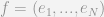
A tensor of type (n, m−n) is an assignment of a multidimensional array $T^{i_1\dots i_n}_{i_{n+1}\dots i_m}[\mathbf{f}]$ to each basis $f = (e_1,...,e_N)$ such that, if we apply the change of basis $\mathbf{f}\mapsto \mathbf{f}\cdot R = \left( R_1^i \mathbf{e}_i, \dots, R_N^i\mathbf{e}_i\right)$ then the multidimensional array obeys the transformation law $T^{i_1\dots i_n}_{i_{n+1}\dots i_m}[\mathbf{f}\cdot R] = (R^{-1})^{i_1}_{j_1}\cdots(R^{-1})^{i_n}_{j_n} R^{j_{n+1}}_{i_{n+1}}\cdots R^{j_{m}}_{i_{m}}T^{j_1,\ldots,j_n}_{j_{n+1},\ldots,j_m}[\mathbf{f}]$ .

A tensor field then is a way to map a tensor to each point of a manifold (the tensor is wrt the tangent space at that point).

When we switch from tensors to tensor fields a new object becomes important: the coordinate system. Before proceeding, one must know what a manifold and a tangent space mean. Then we can illuminate the relation between what one calls a “basis” when speaking about tensors and the “coordinate system” in the context of tensor fields. Firstly, a coordinate system gives a way to continuously map a tuple of numbers to a point on the manifold. This continuous map is what physicist love to work with (Cartesian or polar coordinates for instance). The nice thing is that each coordinate system brings with itself a canonical basis for each point of the manifold.

What can be confusing, is that the basis can change from point to point. For example, one can take the $R^2$ manifold that has $R^2$ as its tangent space. Take for instance two points $(x=1, y=0)$ and $(x=0, y=1)$ . The basis vectors in the Cartesian coordinate system are the same for both points: $(e_x, e_y)$ . However in the polar coordinate system the basis vectors for the first point are $(e_x, e_y)$ and $(e_y, -e_x)$ for the second point.

Anyway, the only thing that changes in the definition, is that the change-of-basis matrix mentioned above now depends on the coordinate systems.

$\hat{T}^{i_1\dots i_n}_{i_{n+1}\dots i_m}(\bar{x}_1,\ldots,\bar{x}_k) = \frac{\partial \bar{x}^{i_1}}{\partial x^{j_1}} \cdots \frac{\partial \bar{x}^{i_n}}{\partial x^{j_n}} \frac{\partial x^{j_{n+1}}}{\partial \bar{x}^{i_{n+1}}} \cdots \frac{\partial x^{j_m}}{\partial \bar{x}^{i_m}} T^{j_1\dots j_n}_{j_{n+1}\dots j_m}(x_1,\ldots,x_k)$

In Terms of Tensor Products

I prefer this definition, as it relies on the geometrical meaning of vectors and forms. According to Wikipedia, one can express it as:

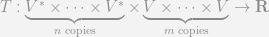
A type (n, m) tensor T is defined as a map $T: \underbrace{ V^* \times\dots\times V^*}_{n \text{ copies}} \times \underbrace{ V \times\dots\times V}_{m \text{ copies}} \rightarrow \mathbf{R}$ , where V is a vector space and V* is the corresponding dual space of covectors, which is linear in each of its arguments.

One can again try to translate this to the case of tensor fields. The straightforward way is just to say that this map is parametrized, thus it depends on which point on the manifold it is evaluated.

However, a more “geometrical” approach would be to keep the part about “a tensor field is the sum of tensor products of vector fields and 1-form fields” but define vector fields and 1-form fields “geometrically”. Vector fields become differential operators over the manifold instead of maps to elements of the tangent space and 1-forms are defined in terms of differentials instead of duals of vectors.

The Magic

The magic is that this parametrization in terms of tuples of real numbers (a coordinate system) brings automatically a canonical basis and and the transformation matrix for change of basis. Hence defining a coordinate system provides a basis for free. Otherwise the generalization of the first definition would have been clumsier.

Leave a comment

by Stefan Krastanov on 09.07.2012 • Permalink

Posted in GSoC - diffgeom, Mathematics

Tagged differential geometry, математика, gsoc, sympy

Posted by Stefan Krastanov on 09.07.2012

https://krastanov.wordpress.com/2012/07/09/tensor-vs-tensor-field-basis-vs-coordinate-system/

Visiting CERN for the Big Announcement

This morning I woke up rather early in order to go to the CERN campus to see the announcement of the new particle for myself. First of all:

Hell, yeah!

Higgs-like particle

When Joe Incandela, the spokeperson for CMS, showed this plot everybody remained silent. He actually forgot to continue his speech for a few moments, sooo happy about being able to show such an insanely cool graph.

Obviously this is a great scientific discovery. Anyhow, it was not a surprise for most physicists, hence I will leave the discussion of the physics out of the way and focus on today’s event itself. (Just to be clear, this is indeed a new particle, however it is not know for sure whether it is the SM Higgs (I will be so happy if it is not (yes, click this link)))

Getting back to the event itself, the atmosphere was indeed great. The conference hall was too small for all the public to fit in, thus, in order to ensure that everybody is happy, CERN had the talks streamed to all meeting rooms on the campus. Regardless, there was a number of enthusiasts that slept in front of the doors to guarantee themselves a place in the main hall. Good for them as it seems that by already 5:30 am there were more than 150 people waiting in front of the hall (the seminar started at 9 o’clock).

After the presentations, the scientists that predicted the particle some 50 years ago were given the opportunity to say a few words. Gerald Guralnik’s comment was very appropriate:

It is wonderful to be at a physics event where there is applause like there is at at football game.

Peter Higgs had tears in his eyes when he said:

It is an incredible thing that it has happened in my lifetime.

In the spirit of these words, we should not forget all the people that were not as lucky and were not able to see the product of their work.

The CERN Director General Rolf Heuer closed the talks by saying:

As a laymen I would now say I think we have it. Do you agree?

And was greeted by ovations from the hall (and all the meeting rooms on campus). This person moderated the talks extremely well. Indeed, it was a pleasure to watch him and the two collaborations’ spokepeople answering the journalists’ questions during the press conference that followed.

Lastly, a few places to check for more information (there is a number of articles on each blog, so check the prev/next buttons):

Leave a comment

by Stefan Krastanov on 04.07.2012 • Permalink

Posted in blah blah, Physics

Tagged CERN, conference, higgs

Posted by Stefan Krastanov on 04.07.2012

https://krastanov.wordpress.com/2012/07/04/visiting-cern-for-the-big-announcement/

Part 1: What is a Tensor and How is it Implemented in the diffgeom SymPy module?

The Math

The notion of “a tensor” is commonly defined in two different ways. The first definition goes roughly like this (“roughly” means “do not tell this to your math teacher”):

A tensor is a geometrical object that can be represented in some coordinate system as an n-dimensional array (it is not the array itself). The quantities in that array depend on the coordinate system in which the representation is done, however there is a precise rule on how these quantities change if we switch to another coordinate system. It is this rule that defines what a tensor (and in particular a vector or a 1-form) is.

The other definition, less used by physicists and more used by mathematicians is (again roughly) the following:

A tensor is the sum of tensor products of forms and vectors. Forms and vectors are themselves given nice geometrical definitions.

It is this second definition that is used in the diffgeom SymPy module. Naturally, we need to define “tensor product”, “vector” and “form” in order to use this definition. Indeed, the structure of the module follows closely these mathematical definitions.

Disclaimer: I have used and will use the words tensor and tensor field interchangeably. In order for this post to make any sense to you, ensure that you understand the difference and are able to find out the exact meaning from the context. The same goes also for vector / vector field and form / form field.

The Implementation

To create the mathematical structure of differential geometry or its implementation in a CAS like SymPy we need to build up the ladder of object definitions. Each new and more interesting notion will depend on the definition of the previous. Hence we start with the boilerplate object “Manifold” and on it we define a “Patch” (the diffgeom module implements all this boilerplate for commonly used manifold, however in order to explain how it works, we will redo everything from scratch):

m = Manifold('my_manifold', 2) # A 2D manifold called 'my_manifold'
p = Patch('my_patch', m) # A patch called 'my_patch'

The first object that does something marginally interesting is the “Coordinate System”. Its role is to permit the parametrization of points on the patch by a tuple of numbers:

cs_r = CoordSystem('R', p) # A coordinate system called 'R' (for rectangular)
point = cs_r.point([1,1]) # A point with coordinates (1, 1)

If you have two or more coordinate systems you can tell the computer how to transform a tuple of numbers from one system to another:

cs_p = CoordSystem('P', p)
cs_r.connect_to(cs_p, [x, y], [sqrt(x**2+y**2), atan2(y,x)])
cs_p.connect_to(cs_r, [r, t], [r*cos(t), r*sin(t)], inverse=False)
# Now the point instances know how to transform their coordinate tuples:
point.coords(cs_p)
# output:
#⎡  ___⎤
#⎢╲╱ 2 ⎥
#⎢     ⎥
#⎢  π  ⎥
#⎢  ─  ⎥
#⎣  4  ⎦

However, differential geometry is not about calculating coordinates of points in different systems. It is about working with fields. Thus, we will focus on a single coordinate system from now on, and to be explicit about its complete independence of whether we want rectangular or other coordinates, we will just call it ‘c’ and leave it unconnected to other coordinate systems.

c = CoordSystem('c', p)

Scalar Field

We continue to build up our ladder of definitions in order to obtain a more interesting and useful theory/implementation. The next step is the “scalar field”. A scalar field is a mapping from the manifold (the set of points) to the real numbers (yes, just reals (maybe complex), the rest brings unnecessary complexity). Each coordinate system brings with itself the basic scalar fields (i.e. coordinate functions), that correspond to the mappings from a point to an element of its coordinate tuple. These basic scalar fields are implemented internally as BaseScalarField instances (this is however invisible to the user).

 c.coord_functions()
# output: [c₀, c₁]
point = c.point([a, b])
c.coord_function(0)(point)
# output: a

You can build more complicated fields by using the base scalar fields. This does not produce an instance of some new ScalarField class. The BaseScalarField instances just become a part of the expression tree of an ordinary Expr instance (the base for building expressions in SymPy).

c0, c1 = c.coord_functions()
field = f(c0, 3*c1)/sin(c0)*c1**2
f
# output:
#               -1       2
#f(c₀, 3⋅c₁)⋅sin  (c₀)⋅c₁
field(point)
# output:
# 2
#b ⋅f(a, 3⋅b)
#────────────
#   sin(a)

Vector Field

Then comes the vector field which is defined as an element of the set of differential operators over the scalar fields. All elements of this set can be build up as linear combinations of base vector fields. The base vector fields correspond to the partial derivatives with respect to the base scalar fields. They are implemented in the BaseVectorField class, which also is invisible to the user.

c.base_vectors()
# output: [∂_c_0, ∂_c_1]
e_c0, e_c1 = c.base_vectors()
e_c0(c0)
# output: 1
e_c0(c1)
# output: 0

One can also use more complicated fields (again, no need for new VectorField class, just being part of the expression tree of Expr):

v_field = c1*e_c0 + f(c0)*e_c1
v_field
# output: f(c₀)⋅∂_c_1 + c₁⋅∂_c_0
s_field = g(c0, c1)
v_field(s_field)
# output:
#      ⎛ d            ⎞│           ⎛ d            ⎞│
#f(c₀)⋅⎜───(g(c₀, ξ₂))⎟│      + c₁⋅⎜───(g(ξ₁, c₁))⎟│
#      ⎝dξ₂           ⎠│ξ₂=c₁      ⎝dξ₁           ⎠│ξ₁=c₀
v_field(s_field)(point)
# output:
#  ⎛ d           ⎞│            ⎛ d           ⎞│
#b⋅⎜───(g(ξ₁, b))⎟│     + f(a)⋅⎜───(g(a, ξ₂))⎟│
#  ⎝dξ₁          ⎠│ξ₁=a        ⎝dξ₂          ⎠│ξ₂=b

1-Form Field and Differential

The final ingredient needed for the basis of differential geometry is the 1-form field. A 1-form field is a linear mapping from the set of vector fields to the set of reals. The interesting thing is that all 1-forms can be build-up from linear combinations of the differentials of the base scalar fields.

There is the need to define what a differential is. The differential $df$ of the scalar field $f$ is the 1-form field which has the following property: for every vector field $v$ one has $df(v) = v(f)$ .

In the diffgeom module the differential is implemented as the Differential class. The differentials of the base scalar fields are accessible with the base_oneforms() method, however one can construct the differential of whatever scalar field they wish. There is, as always, no dedicated OneFormField class. Everything is build up with Expr instances.

c.base_oneforms()
# output: [ⅆ c₀, ⅆ c₁]
dc0, dc1 = c.base_oneforms()
dc0(e_c0), dc1(e_c0)
# output: (1, 0)

And building up more complicated expressions:

f_field = g(c0)*dc1 + 2*dc0
f_field(v_field)
# output: g(c₀)⋅f(c₀) + 2⋅c₁

The Rest

Now that we have the basic building blocks in order to construct higher order tensors we use tensor and wedge products. More about them in part 2.

What if I Need to Work with a Number of Different Coordinate Systems

The only difference is that the chain rule of differentiation will be necessary. One can express the same statement in a more implementation independent way as “The rule for transformation of coordinates will need to be applied”. Anyhow, it works:

Examples from the already implemented $R^2$ module.

Points Defined in one Coordinate System and Evaluated in Another

point_r = R2_r.point([x0, y0])
point_p = R2_p.point([r0, theta0])
R2.x(point_r)
# output: x₀
R2.x(point_p)
# output: r₀⋅cos(θ₀)
trigsimp((R2.x**2 + R2.y**2 + g(R2.theta))(point_p))
# output:
#  2
#r₀  + g(θ₀)

Vector Fields Operating on Scalar Fields

R2.e_x(R2.theta)
# output:
#            -1
#   ⎛ 2    2⎞
#-y⋅⎝x  + y ⎠
R2.e_theta(R2.y)
# output: cos(θ)⋅r

1-Form Fields Operating on Vector Fields

R2.dr(R2.e_x)
# output:
#         -1/2
#⎛ 2    2⎞
#⎝x  + y ⎠    ⋅x

What if I Need an Unspecified Arbitrary Coordinate System

If it is just one coordinate system, nothing; all the examples in the first part were for a completely arbitrary system. If you want two systems with an arbitrary transformation rules between them, just use an arbitrary function when you connect them:

m = Manifold('my_manifold', 2)
p = Patch('my_patch', m)
cs_a = CoordSystem('a', p)
cs_b = CoordSystem('b', p)
cs_a.connect_to(cs_b, [x, y], [f(x,y), g(x,y)], inverse=False)
cs_a.base_vector(1)(cs_b.coord_function(0))
# output:
#⎛ d            ⎞│
#⎜───(f(a₀, ξ₁))⎟│
#⎝dξ₁           ⎠│ξ₁=a₁

How Does This Relate to the Scheme Code by Gerald Jay Sussman and Jack Wisdom

The diffgeom module is based in its entirety on the work of Gerald Jay Sussman and Jack Wisdom on “Functional Differential Geometry”. The only substantial difference (in what is already implemented) is how the diffgeom module treats operations on fields. Both the diffgeom module and the original Scheme code behave like this:

scalar_field(point) ---> an expression representing a real number

However, the original scheme implementation and the SymPy module behave differently in these cases:

 vector_field(scalar_field)
form_field(vector_field)

As far as I know, the original Scheme code produces an opaque object. It indeed represents a scalar field, however $\partial_x(x)$ will not produce directly $1$ . Instead it produces an object that returns 1 when evaluated at a point. The diffgeom module does this evaluation at the time at which one calls $\partial_x(x)$ without the need to evaluate at a point, thus the result is explicit and not encapsulated in an opaque object.

4 Comments

by Stefan Krastanov on 30.06.2012 • Permalink

Posted in GSoC - diffgeom

Tagged differential geometry, gsoc, symbolic algebra, sympy

Posted by Stefan Krastanov on 30.06.2012

https://krastanov.wordpress.com/2012/06/30/part-1-what-is-a-tensor-and-how-is-it-implemented-in-the-diffgeom-sympy-module/

Printing in SymPy (for the Differential Geometry Module)

This week I was doing some interesting refactoring, that brings quite a bit of new possibilities, however I will write about this in the coming days. For now… printing. Most importantly, any suggestions for improvements are very welcomed.

Printing in SymPy is done really easily. You just add a _print_Whatever() method to the printer and your new class is printed in whatever manner you wish.

For the moment I am printing scalar fields just as the name of the coordinate in bold non-italic, vector fields as $\partial$ with the name as a subscript and differentials as a fancy $d$ followed by the name.

First of all the unicode printer:

There are some obvious problems, like the fact that in unicode there is no subscript for $\theta$ or $y$ .

And then the $\LaTeX$ printer:

Now I must find a nice way to print a Point() instance.

Leave a comment

by Stefan Krastanov on 25.06.2012 • Permalink

Posted in GSoC - diffgeom

Tagged differential geometry, gsoc, printing, symbolic algebra, sympy

Posted by Stefan Krastanov on 25.06.2012

https://krastanov.wordpress.com/2012/06/25/printing-in-sympy-for-the-differential-geometry-module/

Integral Curves of Vector Fields in SymPy

A week or two ago I implemented some basic functionality for work with integral curves of vector fields. However, I needed to make additional changes in other parts of SymPy in order for the ODE solver to work with systems of equations and with initial conditions. I also wanted to get my plotting module merged so I can show some visualizations if necessary.

Now that all this is ready (even though not everything is merged in SymPy master) I can show you some of the most basic capabilities implemented in the differential geometry module. First, we start with the boilerplate:

A Simple Field

from sympy.diffgeom import *
from sympy.diffgeom.Rn import * # This gives me:
                                    #   - R2_p - the polar coord system
                                    #   - R2_r - the rectangular coord system
                                    #   - x,y,r,theta - the base scalar fields
                                    #   - e_x, ... - the base vector fields
# Define some fields to play with
# (these are the same fields, defined in two different ways):
vector_field_circular_p = R2_p.e_theta
vector_field_circular_r = -R2.y*R2.e_x + R2.x*R2.e_y
# Define the same point in two different ways
point_p = R2_p.point([1,pi/2])
point_r = R2_r.point([0,1])

The r index is for rectangular coordinate systems and the p index is for polar.

Now using intcurve_diffequ we can generate the differential equations for the integral curve. This function also generates the required initial conditions:

#        vector field      free parameter for    starting point
#                  |        the curve     |     /          coord system
#                  v                      v    v      v-- for the equation
intcurve_diffequ(vector_field_circular_p, t, point_p, R2_p)
# output:
#   d            d
#([ ──(f₀(t)),   ──(f₁(t)) - 1  ],
#   dt           dt
#
#                        π
# [f₀(0) - 1,    f₁(0) - ─      ])
#                        2

intcurve_diffequ(vector_field_circular_p, t, point_p, R2_r)
# output:
#           d                     d
#([ f₁(t) + ──(f₀(t)),   -f₀(t) + ──(f₁(t))  ],
#           dt                    dt
#
# [ f₀(0),               f₁(0) - 1           ])

Here we have equations for the functions $f_0$ and $f_1$ which are by convention the names that intcurve_diffequ gives for the first and second coordinate.

The cool thing is that we can mix the coordinate systems in any way we wish. The code will automatically make the needed coordinate transformation and return the equations in the demanded coordinate system independently of the coordinate systems in which the input objects were defined (at worst you will need to call some simplification routines):

a = intcurve_diffequ(vector_field_circular_p, t, point_p, R2_r)
a == intcurve_diffequ(vector_field_circular_p, t, point_r, R2_r)
# True
a == intcurve_diffequ(vector_field_circular_r, t, point_r, R2_r)
# True
a == intcurve_diffequ(vector_field_circular_r, t, point_p, R2_r)
# True

Solving the equations actually gives (this solver is not yet in SymPy master as of the time of writing):

equ_r, init_r = intcurve_diffequ(vector_field_circular_r, t, point_r, R2_r)
sol_r = dsolve(equ_r+init_r, [Function('f_0')(t), Function('f_1')(t)])
[simplify(s.rewrite(sin)) for s in sol_r] # some simplification
#[f₀(t) = -sin(t), f₁(t) = cos(t)]            # is necessary because
                                              # dsolve returned complex
                                              # exponentials

Even simpler:

equ_p, init_p = intcurve_diffequ(vector_field_circular_p, t, point_p, R2_p)
dsolve(equ_p+init_p, [Function('f_0')(t), Function('f_1')(t)])
# output:
#[f₀(t) = 1,
#             π
# f₁(t) = t + ─
#             2]

This is obviously just a circle (did I mentioned that the vector field that I defined is circular). There is no need to plot it as it is fairly simple. However a slight change will render the field a bit more interesting:

Radial Component

# A circular field that also pushes in radial direction
# towards an equilibrium radius.
v_field = R2.e_theta + (r0 - R2.r)*R2.e_r
# An initial position slightly away from the
# equilibrium one.
start_point = R2_p.point([r0+delta, 0])
equ, init = intcurve_diffequ(v_field, t, start_point)
equ
#                d            d
#[ -r₀ + f₀(t) + ──(f₀(t)),   ──(f₁(t)) - 1 ]
#                dt           dt

init
#[-δ - r₀ + f₀(0), f₁(0)]

dsolve(equ+init, [Function('f_0')(t), Function('f_1')(t)])
#            -t
#[f₀(t) = δ⋅ℯ   + r₀, f₁(t) = t]

This gives a spiral tending towards the equilibrium radius $r_0$ . Let us extract the coordinates from these equations and plot the resulting curve:

intcurve_coords = [eq.rhs for eq in dsolve(equ+init, [Function('f_0')(t), Function('f_1')(t)])]
intcurve_coords
#    -t
#[δ⋅ℯ   + r₀, t]

# We need this in Cartesian coordinates for the plot routine.
# We could have solved for Cartesian coordinates since the
# beginning, however our current approach permits us to see
# how to use the `CoordSys` classes to change coordinate systems:
coords_in_cartesian = R2_p.point(intcurve_coords).coords(R2_r)
coords_in_cartesian
#⎡⎛   -t     ⎞       ⎤
#⎢⎝δ⋅ℯ   + r₀⎠⋅cos(t)⎥
#⎢                   ⎥
#⎢⎛   -t     ⎞       ⎥
#⎣⎝δ⋅ℯ   + r₀⎠⋅sin(t)⎦

# Substitute numerical values for the plots:
x,y = coords_in_cartesian.subs({delta:0.5, r0:1})
plot(x,y, (t,0,4*pi))
#Plot object containing:
#[0]: parametric cartesian line:
#      ((1 + 0.5*exp(-t))*cos(t), (1 + 0.5*exp(-t))*sin(t))
#      for t over (0.0, 12.566370614359172)

This is all great, but what happens if one has to work with more complicated fields. For instance the following simple field will not permit analytical solution:

No Analytical Solution

v_field = R2.e_theta + r0*sin(1 - R2.r/r0)*R2.e_r
equ, init = intcurve_diffequ(v_field, t, start_point)
equ
#[
#        ⎛    f₀(t)⎞   d
#- r₀⋅sin⎜1 - ─────⎟ + ──(f₀(t))
#        ⎝      r₀ ⎠   dt       ,
#
#d
#──(f₁(t)) - 1
#dt           ]

For cases like this one the user can take advantage of one of the numerical ODE solvers from scipy. Or sticking to symbolic work he can use the intcurve_series function that gives the series expansion for the curve:

intcurve_series(v_field, t, start_point, n=1)
#⎡δ + r₀⎤
#⎢      ⎥
#⎣  0   ⎦

intcurve_series(v_field, t, start_point, n=2)
#⎡            ⎛    δ + r₀⎞     ⎤
#⎢δ + r₀⋅t⋅sin⎜1 - ──────⎟ + r₀⎥
#⎢            ⎝      r₀  ⎠     ⎥
#⎢                             ⎥
#⎣              t              ⎦

intcurve_series(v_field, t, start_point, n=4, coeffs=True)
#[
#⎡δ + r₀⎤
#⎢      ⎥
#⎣  0   ⎦,
#
#⎡        ⎛    δ + r₀⎞⎤
#⎢r₀⋅t⋅sin⎜1 - ──────⎟⎥
#⎢        ⎝      r₀  ⎠⎥
#⎢                    ⎥
#⎣         t          ⎦,
#
#⎡     2    ⎛    δ + r₀⎞    ⎛    δ + r₀⎞⎤
#⎢-r₀⋅t ⋅sin⎜1 - ──────⎟⋅cos⎜1 - ──────⎟⎥
#⎢          ⎝      r₀  ⎠    ⎝      r₀  ⎠⎥
#⎢──────────────────────────────────────⎥
#⎢                  2                   ⎥
#⎢                                      ⎥
#⎣                  0                   ⎦,
#
#⎡      ⎛     2                  2            ⎞                ⎤
#⎢    3 ⎜      ⎛    δ + r₀⎞       ⎛    δ + r₀⎞⎟    ⎛    δ + r₀⎞⎥
#⎢r₀⋅t ⋅⎜- sin ⎜1 - ──────⎟ + cos ⎜1 - ──────⎟⎟⋅sin⎜1 - ──────⎟⎥
#⎢      ⎝      ⎝      r₀  ⎠       ⎝      r₀  ⎠⎠    ⎝      r₀  ⎠⎥
#⎢─────────────────────────────────────────────────────────────⎥
#⎢                              6                              ⎥
#⎢                                                             ⎥
#⎣                              0                              ⎦]

However these series do not always converge to the solution, so care should be taken.

There are other amusing possibilities already implemented, however I will write about them another time.

If you want to suggest more interesting examples, please do so in the comments.

Leave a comment

by Stefan Krastanov on 17.06.2012 • Permalink

Posted in GSoC - diffgeom

Tagged differential geometry, gsoc, integral curve, symbolic algebra, sympy, vector analysis, vector field

Posted by Stefan Krastanov on 17.06.2012

https://krastanov.wordpress.com/2012/06/17/integral-curves-of-vector-fields-in-sympy/

Consistent output from the SymPy solvers (and some ideas about the ODE solver)

The work on the differential geometry module has not progressed much this week. I have fixed some minor issues, docstrings and naming conventions, however I have not done much with respect to the implementation of form fields as there are still some questions about the design to be ironed out.

Instead I focused on studying two of the features that SymPy presents and that I will use heavily. The first is the simplification routine that I will discuss another time. The second one is the different solvers implement in SymPy.

First of all, I have a very hard time getting used to the various output that the solvers provide. The algebraic equations solver, for example, can return either an empty list or a None instance if there is no solution. If there are solutions it can return a list of tuples of solutions, or a list of dictionaries of solutions, or a list of solutions if there is only one variable to solve for, or the solution itself if the solution is unique… Thankfully, a remedy for this was implemented by Christopher Smith. In pull request 1324 he provided some flags that force the solver to return the solutions in a canonical form. I am very grateful for his work and I hope that in the not too distant future what he has done will become the default behavior. I also hope that the solver will get refactored, because internally it is still a mess of different possible outputs that are canonicalized only at the very end. It is possible that I will work on this later.

Then there is the ODE module. I already need this solver in order to work with the integral curves that my code produces[1]. It is a very advanced solver written a few years ago by Aaron Meurer as part of his GSoC project. However, it still does not support systems of ODEs or solving for initial conditions. With Aaron’s help I have started those. The main difficulty is that I am covering only the simplest cases, however the new API must be futureproof. Moreover, here I again have a problem with the various outputs that can be produced by the ODE solver. Solutions are always returned as Equation instances (which is necessary, as some solutions can be in implicit form), however if there are multiple solutions they are returned in a list, while single solutions are returned themselves (not in a list). Anyway, the structure of the ODE module is straightforward so this should not be too hard to work around.

This week I will probably finish my work with the ODE solver and proceed to the form fields.

[1] The code on the differential geometry side is ready, however before showing it I will first extend the ODE solver in order to have more interesting examples.

Leave a comment

by Stefan Krastanov on 04.06.2012 • Permalink

Posted in GSoC - diffgeom

Tagged differential geometry, gsoc, ode, solver, symbolic algebra, sympy

Posted by Stefan Krastanov on 04.06.2012

https://krastanov.wordpress.com/2012/06/04/consistent-output-from-the-sympy-solvers-and-some-ideas-about-the-ode-solver/

Scalar and Vector Fields in SymPy – First Steps

The Differential Geometry module for SymPy already supports some interesting basic operations. However, it would be appropriate to describe its structure before giving any examples.

First of all, there are the Manifold and Patch classes which are just placeholders. They contain all the coordinate charts that are defined on the patch and do not provide, for instance, any topological information. This leads us to the CoordSystem class which contains all the coordinate transformation logic. For example, if I want to define the $\mathbb{R}^2$ euclidean manifold together with the polar and Cartesian coordinate systems I would do:

R2 = Manifold('R^2', 2)
# Patch and coordinate systems.
R2_origin = Patch('R^2_o', R2)
R2_r = CoordSystem('R^2_r', R2_origin)
R2_p = CoordSystem('R^2_p', R2_origin)

# Connecting the coordinate charts.
x, y, r, theta = [Dummy(s) for s in ['x', 'y', 'r', 'theta']]
R2_r.connect_to(R2_p, [x, y],
                      [sqrt(x**2 + y**2), atan2(y, x)],
                inverse=False, fill_in_gaps=False)
R2_p.connect_to(R2_r, [r, theta],
                      [r*cos(theta), r*sin(theta)],
                inverse=False, fill_in_gaps=False)

All following examples will be about the $\mathbb{R}^2$ manifold which is already implemented in the code for the module. Also, notice the use of the inverse and fill_in_gaps flags. When they are set to True the CoordSystem classes try to automatically deduce the inverse transformations using SymPy’s solve function.

Now that we have a manifold we would like to create some fields on it and define some points that belong to the manifold. The points are implemented in the Point class. You need to specify some coordinates when you define the point, however after that the object is completely coordinate-system-idependent.

# You need to specify coordinates in some coordinate system
p = Point(R2_p, [r0, theta0])

Then one can define fields. ScalarField takes points to real numbers and VectorField is an operator on ScalarField taking a scalar field to another scalar field by applying a directional derivative. For example, here x and y are the scalar fields taking a point and returning it’s coordinate and d_dx and d_dy are the vector fields $\frac{\partial}{\partial x}$ and $\frac{\partial}{\partial y}$ . R2_r is the Cartesian coordinate system and R2_p is the polar one.

R2_r.x(p) == r0*cos(theta0)
# R2_r.d_dx(R2_r.x) is a also scalar field
R2_r.d_dx(R2_r.x)(p) == 1

Looking at how can these fields be defined:

# For a ScalarField you provide the transformation in some coordinate system
R2_r.x = ScalarField(R2_r, [x0, y0], x0)
#                     /      |        ^-------- the result
#     the coord system     the coordinates

# For a VectorField you provide the components in some coordinate system
R2_r.d_dx = VectorField(R2_r, [x0, y0], [1, 0])
#                        /      |         ^-------- the components
#         the coord system     the coordinates

Obviously one can define much more interesting fields. For instance the potential due to a point charge at the origin is:

potential = ScalarField(R2_p, [r0, thata0], -1/r0)
# And to reiterate, the definition does not limit you
# to use it only in this coordinate system. For instance:
potential(R2_r.point([x0, y0])) == 1/sqrt(x0**2 + y0**2)

However there is another more intuitive way to do it:

# R2_p.r is the scalar field that takes a point and returns the r coordinate
potential2 = 1/R2_p.r
potential2(R2_r.point([x0, y0])) == 1/sqrt(x0**2 + y0**2))

And this new object potential2 is not an instance of ScalarField. It is actually a normal SymPy expression tree that contains a ScalarField somewhere in its leafs (namely in this case it is Pow(R2_p.r, -1)). However, due to the change to one of the base classes of SymPy that I did in this pull request it is now possible for such tree to be a python callable, by recursively applying the argument to each callable leaf in the tree. This change is still debated and it may be reverted.

Vector fields can also be build in this manner. However, they pose a problem. What happens when you multiply a vector field and a scalar field? This operation should give another vector field. And here is a possible problem with the approach of recursively callable expressions trees:

# Naively this operation will call a scalar field on
# another scalar field which is nonsense:
(R2_r.x * R2_r.d_dx)(R2_r.x) == R2_r.x(R2_r.x) * R2_r.d_dx(R2_r.x)
#                         nonsense----^

The current solution is for scalar_field(not_point) to return the callable itself. Thus we have:

(R2_r.x * R2_r.d_dx)(R2_r.x) == R2_r.x * R2_r.d_dx(R2_r.x)
#\________________/ \______/    \_______________________/
#   vector field        ^---scalar fields---^

This way there is no need for complicated logic in __mul__ nor is there need for addition subclasses of Expr in order to accommodate this behavior.

There is not much more to be said about the structure of the module. There are some other nice things already implemented like integral curves, however I will discuss these in a later post.

Among the things that should be done at some point:

Should vector fields be callable on points? If yes, what the result should be? An abstract vector, a tuple of coordinates in a certain coordinate system, something else?
There are many expressions generated by this code that are not simple enough. I should work on the simplification routines and on the differential geometry module itself in order to get more canonical expressions.
The last point is also valid about the solvers: some coordinate transformations are too complicated for the solvers to find the inverse transformation.
Manifold and Patch have name attributes. Are these necessary? What is the role of name attributes in SymPy besides printing?
Start using Lambda where applicable.
Follow better the class structure of SymPy.

Leave a comment

by Stefan Krastanov on 27.05.2012 • Permalink

Posted in GSoC - diffgeom

Tagged differential geometry, gsoc, integral curve, scalar field, symbolic algebra, sympy, vector field

Posted by Stefan Krastanov on 27.05.2012

https://krastanov.wordpress.com/2012/05/27/scalar-and-vector-fields-in-sympy-first-steps/

Differential Geometry in SymPy – my GSoC project

The next few moths will be interesting. I got accepted in the Google Summer of Code program and I am already starting to worry (irrationally) about the project and the schedule. I will be working on a differential geometry module for SymPy (and time permitting, some more advanced tensor algebra).

Basically, I want to create the boilerplate that will permit defining some scalar/vector/form/tensor field in an arbitrary coordinate system, then doing some coordinate-system-independent operations on the field (with hopefully coordinate-system-independent simplifications) and, finally, getting the equations describing the final result in another arbitrary coordinate system.

With this in mind, the details about the project can be seen on the proposal page. Most of it (all except the tensor algebra that I may work on at the end) is based on the work of Gerald Jay Sussman and Jack Wisdom on “Functional Differential Geometry”. I suppose that this project started as a part of their superb book “Structure and Interpretation of Classical Mechanics” (I really have to read this book if I am to call myself a physicist) and the accompanying “Scheme Mechanics” software. By the way, reading the Scheme code is a wonderful experience. This language is beautiful! The authors are also actively updating their code and a newer, more detailed paper on the project can be found here.

Most of my work will be reading the Scheme code and tracing corner cases in SymPy. My workflow will probably consist of implementing some notion from “Functional Differential Geometry” in SymPy and only when I get to semi-working state comparing with the original Scheme code for ideas, then repeating the process on the next part of the system. This way I will be less susceptible to implementing Scheme idioms in Python.

Writing the final version of each function/class of my module will probably take very little time. Most of the time will be dedicated to removing/studying corner cases and assumptions in SymPy’s codebase (more about these later) and experimenting with different approaches for the module structure (and of course reading/deciphering the work of Wisdom and Sussman).

Finally, I will speak a bit about the aforementioned corner cases and assumptions in the SymPy’s codebase. There are the obvious things like having to derive from Expr if you want to be able to have your class as a part of a symbolic expression. Then there is the fact that Basic (and its subclasses like Expr) do some magic with the arguments for the constructor (saved in expr._args) in order to automagically have:

rebuildable expression with eval(srepr(expr))==expr
rebuildable expression with type(expr)(*expr._args)
some magic with the _hashable_content() method in order to (presumably) have efficient cashing

These details make it a bit unclear how to implement things like CoordinateSystem objects which learn during their existence how to transform to other coordinate systems (thus their implementation in code is a mutable object) but at the same time they are the same mathematical object. Anyway, from what I have seen just having a persistent hash and a correct srepr should be enough. I wonder how tabu it is to change your _args after the creation of the class. Why I need to worry about caching (thus the hash) and rebuilding (thus the srepr) is still unclear to me, but I will dedicate whole posts to them later on when I have the explanation. The caching is presumably for performance. It is the need for all that fancy magic that does not permit duck typing in SymPy. If you do not subclass Basic, you can not be part of SymPy, no matter the interfaces that you support.

Then there is the question of using the container subclasses of Expr. Things like Add and Mul, which I would have expected to be just containers. However, they are not. They also do some partial canonicalization, but at the moment their exact role (and more importantly, what they don’t do) is very unclear to me. There was much discussion about AST trees and canonicalization on the mailing list, if you are interested, and how exactly to separate the different duties that Add and Mul have, but as this is enough work for another GSoC I decided to just stop thinking about that and use them in the simples way possible: just as containers.

There is one drawback to this approach. The sum of two vector fields for example is still a vector field and the object that represents the sum should have all the methods of the object representing one of the fields, however Add does not have the same methods as VectorField. The solution that was already used in the matrix module was to create classes like MatrixAdd, and the same was done in the quantum physics module. However, I fear such proliferation of classes for it becomes unsustainable as the number of different modules grows. What happens when I want to combine two objects from the disjoint modules? This is why I simply use Add and Mul and implement helper functions that are not part of the class. These helper functions will ideally be merged in some future canonicalizer that comes about from separating the container and canonicalization parts of Add and Mul.

One last remark is that I will probably have to work on sympify and the sympification of matrices, as I will use coordinate tuples (column vectors) quite often. Then there is the distinction between Application and Function and all the magic with metaclasses that seems very hard to justify. But probably I will write entire posts in which I try to understand why the metaclasses in the core are necessary.

1 Comment

by Stefan Krastanov on 14.05.2012 • Permalink

Posted in GSoC - diffgeom

Tagged differential geometry, gsoc, symbolic algebra, sympy, vector analysis

Posted by Stefan Krastanov on 14.05.2012

https://krastanov.wordpress.com/2012/05/14/differential-geometry-in-sympy-my-gsoc-project/

Some Fractal Renderings

Quite some time ago I decided to learn how to program idiomatically in C++. A great resource were the C++ Annotations by Frank B. Brokken, which by the way are also in Debian’s repositories.

My first and only project in C++ was to write a fractal renderer. I wanted to do something idiomatic, so I started creating classes upon classes abstracting everything that I can think of (the function to be iterated, the convergence criterion, the visualization method, etc). At the end I got something interesting, working and amusing. However I am not sure whether I reached the goal of getting it done idiomatically. Moreover, the program is certainly on the lower end performance-wise.

Anyhow, here is what it was capable of:

Mandelbrot fractals of any order ( $z_{n+1}=z_n^p + c$ for any $p$ and not just 2), Mandelbar fractal, etc.
The dual Julia fractals.
Various coloration schemes.
Superimposing Julia fractals over the Mandelbrot fractals.
Getting some quite useless 3D visualizations.
Getting feedback on the convergence.
Zooming and panning of course.

One drawback is that I based the image manipulation and the GUI event loop on CImg, which was an overkill and its api is constantly in a flux. Hence I have to fix the api calls every time when I want to compile the code as this is once every few years and I can never find the version of CImg for which the original was written.

The code can be found on my gitorious page.

And here are some renderings.

The last one that seem grainy are actually downscaled superpositions of Julia over Mandelbrot fractals. You may try to zoom on them. The original was 10000×10000 pixels.

Leave a comment

by Stefan Krastanov on 02.04.2012 • Permalink

Posted in Computing, Mathematics

Tagged C++, fractals

Posted by Stefan Krastanov on 02.04.2012

https://krastanov.wordpress.com/2012/04/02/some-fractal-renderings/

Kernel parameters make a difference in power consumption

Yeah, obviously. Some time ago I bought a WeTab portable computer and the machine is wonderful. I can (and I actually do) use it in any way imaginable: it’s a tablet form factor (so it’s my heavy ebook reader) and with Ubuntu installed it is also my primary workstation (for CPU heavy stuff I ssh to a server). But the battery life is 4-5 hours tops. And with the recent ASPM problems in the kernel it got worse. But Phoronix already proposed a solution in the form of a few kernel parameters in a very useful article a few months ago.

Here are the results from the WeTab. It translates to about 20 minutes.

Leave a comment

by Stefan Krastanov on 05.12.2011 • Permalink

Posted in Computing

Tagged linux, phoronix, power usage, wetab

Posted by Stefan Krastanov on 05.12.2011

https://krastanov.wordpress.com/2011/12/05/kernel-parameters-make-a-difference-in-power-consumption/

Какво смята обменен студент от Yale University за Препа

Yale е сред най-добрите университети в света (не са чак толкова добри по физика) и учениците там са наясно с това и се гордеят. В тази статия от училищния им вестник студент отишъл на обмен във Франция споделя впечатленията си.

2 Comments

by Stefan Krastanov on 02.12.2011 • Permalink

Posted in Образование във Франция

Tagged обмен, образование, препа, Grandes écoles, Yale

Posted by Stefan Krastanov on 02.12.2011

https://krastanov.wordpress.com/2011/12/02/%d0%ba%d0%b0%d0%ba%d0%b2%d0%be-%d1%81%d0%bc%d1%8f%d1%82%d0%b0-%d0%be%d0%b1%d0%bc%d0%b5%d0%bd%d0%b5%d0%bd-%d1%81%d1%82%d1%83%d0%b4%d0%b5%d0%bd%d1%82-%d0%be%d1%82-yale-university-%d0%b7%d0%b0-%d0%bf/

Скъпоценния камък на Гаус

Есе за скъпоценния камък на Гаус

Leave a comment

by Stefan Krastanov on 23.06.2011 • Permalink

Posted in Есета

Tagged диалог, есе, математика

Posted by Stefan Krastanov on 23.06.2011

https://krastanov.wordpress.com/2011/06/23/%d1%81%d0%ba%d1%8a%d0%bf%d0%be%d1%86%d0%b5%d0%bd%d0%bd%d0%b8%d1%8f-%d0%ba%d0%b0%d0%bc%d1%8a%d0%ba-%d0%bd%d0%b0-%d0%b3%d0%b0%d1%83%d1%81/

Конкурса по Физика на фондация Миню Балкански 2011

Аз бях гордият автор на задачите за конкурса тази година.

Ако не сте млад физик или физичка вероятно не сте чували за него (Всъщност има и конкурс по математика). Но ако сте от моята каста то знаете за претенциите, че конкурсът е на същото високо ниво като националната олимпиада (обикновено тези претенции са напълно обосновани). И както националната олимпиада е пътят за участие в отбора за IPhO, така и конкурсът по физика на фондация Миню Балкански отваря вратите за обучение във френско висше училище (знаехте това… нали?). Но тук ще говоря за задачите които аз дадох и за работите които аз проверих. За детайли относно конкурса погледнете сайта на фондацията.

Задачите (които можете да свалите тук)

Аз съм авторът на първа задача. Втората е дело на Светослав Чакъров с доста промени от моя страна. И двете задачи бяха под редакторския контрол на Янко Тодоров.

Ще започна от втора задача – съвсем кратко защото не съм аз авторът. Смятам я за по-лесна от моята задача, но условието със сигурност е по-плашещо. За първия въпрос е достатъчно да се знае най-основния закон в термодинамиката и да се приложи сляпо. След това внимателно четене и базови познания по метод на размерностите е достатъчен, за да се реши. Задачата намеква за интересни “философски” въпроси, но те са много далече извън обсега на знанията очаквани от състезателите.

А фактът, че от 12 състезателя двама са я решили изцяло, а останалите почти не са я погледнали, смятам че е доказателство че е “по-лесна от моята задача, но условито със сигурност е по-плашещо”.

Първа задача – вълнова оптика

Задачата започва със стряскащо заглавие “Фурие трансформации и филтрация на пространствени честоти”. Но в нито един момент не се очаква от участниците да знаят какво значат тези термини. Темата е как вълновата оптика позволява да се филтрират дадени елементи от изображение.

Задачата може да се раздели на две части. Първа част е с доста сметки. Но съвсем стандартни сметки, доказващи базови свойства на дифракционните решетки.

Само първенката е успяла да спомене нещо относно този закон, при това подозирам, че е имала късмет да го знае наизуст (което всъщност бих очаквал от всички участници) защото е забравила един много важен множител (в който се крие цялата идея). В защита от тези които биха казали “че това не е физика, това са скучни сметки…” ще отговоря, че решението можеше да се намери с “рисуване на стрелки” и чисто “физически” разсъждения. Това е причината въпросното момиче да получи все пак част от точките, въпреки грешно наизустена формула – дала е обяснението в което се крие красотата на идеята.

И каква е тази идея? Главно как се увеличава спектралната разделителна способност на дифракционна решетка когато се увеличи броя на процепите. Знание за критерия на Релей и за разликата между дифракционна решетка и експеримента на Юнг биха били предостатъчни, за да се досети човек какво е решението. Но май повечето от участниците не са били напълно способни да интерпретират дифракционна картина. Жалко, намирам че такова упражнение доставя голямо интелектуално удоволствие.

Но единственото което е нужно, за да може да се продължи към втората половина е [тук цитирам единствената друга дама от участниците и единствената която е използвала толкова невероятно точно описание на вълновите феномени] “The angular spacing of the features in the diffraction pattern is inversely proportional to the dimensions of the object causing the diffraction. In other words: the smaller the diffraction [grating] is, the wider the resulting diffraction pattern, and vice versa.” Това всъщност е фундаментално и много красиво свойство на фурие трансформациите и от там идва ефекта, който се наблюдава в оптиката (дифракция) и в квантовата механика (неравенството на Хайзенберг).

И сега втората част от моята задача. Дадена е снимка на перо:

credit Wikipedia

И е зададен въпроса: “Какво трябва да се направи, за да се получи образ съдържащ само основните косъмчета, но в който най-дребните “барбули” липсват?”.

След това е показан снимка на стена:

credit Wikipedia

И е зададен въпроса: “Какво трябва да се направи да се премахне дефекта при снимане (вълновата структура в долния десен ъгъл)?”.

Участниците трябва да се сетят какво причинява ефекта и да измислят как да го контрират (погледнете цитата в горния абзац). Никой не е предложил успешен подход (повечето не са предложили никакъв подход). Има само едно интересно предложение включващо дълга тръба и още няколко детайла, но даже то беше прекалено далече от работещо решение.

А щях да съм толкова радостен ако някой беше решил интересната част от моята задача (тъжен Стефо)…

Класиране

За щастие беше лесно да се отделят първите двама (защото само двама биват поканени в Париж):

Точки по първа задача

Точки по втора задача

Общ резултат

Много по интересно е кой е първи:

Година на завършване срещу резултат (повечето хора биха очаквали хиперболична зависимост...)

Една много млада дама. Фактът че е малка беше достатъчно учудване. Но още по-рядко девойки решават да се занимават с физика. Резултатите които е изкарала (първа със забележима преднина) много ме радват. Повече момичета в България трябва да видят този комикс.

Бисери

Естествено че имаше…

Много се чудех дали да ги оставя анонимни. Ще направя следния компромис. Издавам, че някои от бисерите са на първенците:

Принципа на Хайзенберг може да се запише като $dE dt\approx\hbar$

Нечестен съм да включвам това, първо защото искахме подобно разсъждение, второ защото всички зайци се очаква да го наизустяват, но интересното че доказателството на това неравенство е различно от доказателството на неравенството на Хайзенберг. Отделно, тъй като това твърдение е наизустено, никой не се опитва да обясни как така от неопределеност отиваме до абсолютна стойност на импулса/енергията/координатата на частица.

Предложено решение на задачата за перцето:

The feather can be taken for diffraction grating with distance between slits 1mm and lenght of the slits also 1mm […] So the only thing we have to do is to light the feather from enough far distance, because the light must be perpendicular to the feather

Започва добре, но след това загубва работещата идея.

Нещо което много хора бъркат:

A diffraction grating is a grating which has very small holes or slits almost comparable to the wavelenght of light [подчертаното е от мен]

The slits are as big as the length of the wave, which passes throught them.

Да видим каква константа ще има една такава решетка. Брой резки на милиметър ще е $n = \frac{1mm}{500nm} \approx 2000$ . Хъм… не е толкова зле колкото си мислех, но и това е прекалено голям брой. Освен това такава решетка ще има друг проблем – дълбочината ѝ (не широчина или дължина) няма да е пренебрежима и лесната заучена формула няма да е вече приложима.

И сега две от любимите ми:

[относно заснетата тухлена стена] Obviously the dark lines are diffraction minima and the light one – maxima. This effect is seen on TV, too, when somebody wears striped clothes. What occurs is diffraction from round hole (from the objective of the camera) and interference from thin films (the different materials of which lenses in a camera are made) […]

Интересното е, че май тези разсъждения дадоха верен числен резултат. За жалост са грешни (въпреки че са оригинални и интересни) и получават нула точки.

И второто, което малко ме стресна (но много би зарадвало Verlinde (погледни увода на втора задача за контекст)):

Forces of entropic origin are all 4 fundamental forces including gravity and electromagnetic forces.

Една интересна аргументация относно втора задача:

According to the theory of Verlinde the force must be gravity [до тук ок]. It can’t be any of the other fundamental three, because all of them depend on the electric charge and this one doesn’t.

Не твърдя че аргументацията е грешна. Със сигурност е много интересна.

И сега нещо което е много грешно. Имате лазер, дифракционна решетка, леща и екран. Какво трябва да направите за да получите хубав образ на екрана.

Със сигурност не следното:

Правилното решение (и разликата е много дълбока и важна):

Май това е всичко. Приятно прекарване в Париж на двамата първенци и поздрави за неотразимия учител Теодосиев от Казанлък, който е обучил толкова талантлива млада дама (първенката).

Участниците да се чувстват свободни да ми пишат по мейл или в коментарите по-долу. Както и всички които искат подробности относно задачите.

Ако някой от участниците се чувства некомфортно от публикуването на бисерите, без притеснение може да ми пише лично съобщение и да помоли да ги сваля. Но не смятам, че има нещо което да причини притеснение. Всички правим грешки, и най-добре се учим от тях (особено ако се смеем).

Leave a comment

by Stefan Krastanov on 20.06.2011 • Permalink

Posted in Конкурс по Физика "Миню Балкански"

Tagged задачи, класиране, конкурс, състезание, фондация Миню Балкански

Posted by Stefan Krastanov on 20.06.2011

https://krastanov.wordpress.com/2011/06/20/%d0%ba%d0%be%d0%bd%d0%ba%d1%83%d1%80%d1%81%d0%b0-%d0%bf%d0%be-%d1%84%d0%b8%d0%b7%d0%b8%d0%ba%d0%b0-%d0%bd%d0%b0-%d1%84%d0%be%d0%bd%d0%b4%d0%b0%d1%86%d0%b8%d1%8f-%d0%bc%d0%b8%d0%bd%d1%8c%d0%be-%d0%b1/

За обновяване на адресите

In Terms of Transformation Rules

In Terms of Tensor Products

The Magic

The Math

The Implementation

Scalar Field

Vector Field

1-Form Field and Differential

The Rest

What if I Need to Work with a Number of Different Coordinate Systems

Points Defined in one Coordinate System and Evaluated in Another

Vector Fields Operating on Scalar Fields

1-Form Fields Operating on Vector Fields

What if I Need an Unspecified Arbitrary Coordinate System

How Does This Relate to the Scheme Code by Gerald Jay Sussman and Jack Wisdom

A Simple Field

Radial Component

No Analytical Solution

Задачите (които можете да свалите тук)

Първа задача – вълнова оптика

Класиране

Бисери

Categories